From BERTology to PEFT: Notes on an AACL 2022 Tutorial

Hong-Wei Wu included in category Essential AI Concept

2023-09-01 2026-08-23 3323 words 15 minutes

Notes from an AACL 2022 tutorial: what BERT's layers learn, why sentence embeddings need contrastive learning, and how PEFT like LoRA fine-tunes huge models cheaply.

Contents

Title slide of the 2022 AACL Tutorial: Recent Advances in Pre-trained Language Models, listing the tutorial name and speakers — Title slide of the 2022 AACL Tutorial: Recent Advances in Pre-trained Language Models [source: the tutorial’s own first slide]

1 Introduction

These are my notes on the AACL-IJCNLP 2022 Tutorial: Recent Advances in Pre-trained Language Models. The goal is to give anyone who already has basic NLP knowledge, but hasn’t systematically studied Pre-trained Language Models (PLMs), a map of the territory — so I’ve only kept the ideas I found most worth writing down, not a slide-by-slide translation. For the full picture, the tutorial itself has a video and slides.

The whole thing really breaks into three arcs: first, understanding what a PLM actually learns (#1–#4); then, where it learns badly and how to fix that (#5–#8); and finally, what to do once a model is too big to fine-tune in the ordinary way (#9–#13).

#1: Pre-trained Language Models learn Contextualized Word Representations
#2: BERTology — understanding what linguistic knowledge each BERT layer learns
#3: BERT Embryology — understanding what knowledge BERT acquires at each stage of training
#4: Pre-trained Language Models have cross-discipline transfer ability
#5: BERT’s sentence-level representations are a weak spot
#6: Why learning good sentence-level representations matters
#7: BERT-flow and BERT-whitening help BERT produce better sentence representations
#8: Using contrastive learning to help BERT produce better sentence representations
#9: The idea behind Parameter-Efficient Fine-tuning
#10: PEFT: Adapter
#11: PEFT: LoRA (Low-Rank Adaptation of Large Language Models)
#12: PEFT: Prefix Tuning
#13: PEFT: Soft Prompting

2 #1: Pre-trained Language Models Learn Contextualized Word Representations

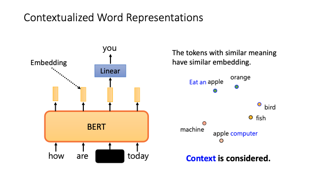
Diagram showing a pre-trained language model taking in a sentence and outputting, for each word, a vector that carries contextual information — What a pre-trained language model learns is a Contextualized Word Representation

Word2vec and GloVe learn Word Representations: each word maps to one fixed vector, retrieved by lookup. A Pre-trained Language Model is different — it learns Contextualized Word Representations, so the same word gets a different representation depending on the context it appears in.

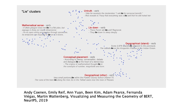
The same word ‘Lie’ appearing in two different sentences, with the model outputting two different representation vectors for each occurrence — The same word takes on different meanings in different contexts, and so produces different representations

The figure above uses “Lie” as the example. It can mean “to tell a falsehood” or “to lie down” — two completely different meanings. In the Word2vec world it only has one vector, so the model has to somehow cram both meanings into a single point. In a PLM, it produces two distinct representations depending on context, which makes life much easier for whatever downstream task comes next.

3 #2: BERTology — What Does Each BERT Layer Actually Learn?

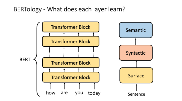
Diagram labeling BERT’s layers from bottom to top, showing surface-level information in the lower layers, syntactic knowledge in the middle layers, and semantic understanding in the top layers — BERT’s earlier layers learn surface-level meaning, the middle layers pick up syntax, and the final layers understand the semantics of the whole sentence

Once we know a PLM learns Contextualized Representations, the next natural question is: where in the model does that knowledge actually live? This line of research is called BERTology.

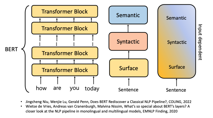
The method is to use probing techniques to analyze what information is contained in the representation output by each of BERT’s layers. Researchers found that the earlier layers mostly capture surface-level linguistic knowledge, the middle layers start to understand “syntax,” and the final layers handle semantics. The paper BERT Rediscovers the Classical NLP Pipeline (ACL'19) puts it even more bluntly: what BERT does from its first layer to its last looks a lot like a traditional NLP pipeline processing a sentence.

That conclusion has since been revised, though. Later work points out that the division of labor isn’t so clean — which layer does what actually shifts depending on the input (shown on the right side of the figure below).

Comparison chart showing how the distribution of linguistic knowledge across a model’s layers shifts under different inputs for the same model — The information each layer of a pre-trained language model learns is affected by the current input

4 #3: BERT Embryology — What Does BERT Learn at Each Stage of Training?

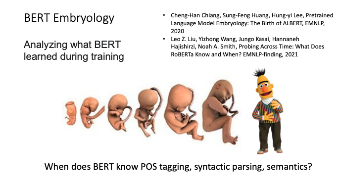
Conceptual diagram with training steps on the x-axis, illustrating that BERT acquires different linguistic abilities at different stages of pre-training — BERT Embryology: understanding what information BERT acquires at different points during training

#2 asked “where in the model is the knowledge stored?” This section asks about a different axis: “at what point in training does the knowledge emerge?” This line of work is called BERT Embryology — a fitting name, since it treats the pre-training process like embryonic development, asking whether the model learns syntax or semantics first.

5 #4: Pre-trained Language Models Have Cross-Discipline Transfer Ability

Flowchart showing a model pre-trained on human language and then fine-tuned on a completely unrelated task such as DNA sequence or protein structure classification — Pre-trained Language Models have cross-discipline transfer ability

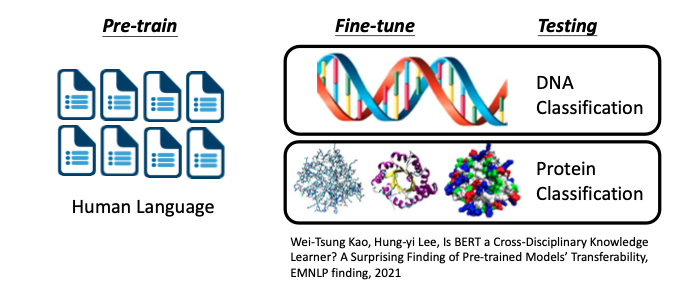
Here’s an interesting experimental setup: pre-train on a large amount of human language, then fine-tune on a task from a completely unrelated domain (e.g. classifying DNA sequences or protein structures). Intuitively, you’d worry that the model picked up a bunch of linguistic knowledge it can’t use, and that this actively hurts it on the downstream task.

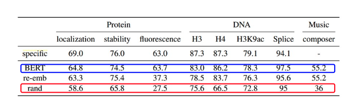
Bar chart comparing the scores of a pre-trained BERT model against a randomly initialized model on cross-domain downstream tasks — A pre-trained model (BERT) still outperforms a randomly initialized model (rand)

The result is the opposite. A model that’s pre-trained and then fine-tuned (BERT) still beats a randomly initialized model that’s fine-tuned directly (rand). A reasonable guess is that what a language model picks up during pre-training isn’t just knowledge specific to that dataset — it also includes some more generalizable ability related to “how to classify a sequence,” which turns out to transfer even to a different domain entirely.

6 #5: BERT’s Sentence-Level Representations Are a Weak Spot

Sections #1 through #4 covered BERT’s strengths. But BERT has a clear weakness too: it’s strong at the word level, and noticeably less impressive at the sentence level.

Bar chart comparing scores of various methods for deriving a sentence representation from BERT against averaged GloVe vectors on a sentence similarity task — BERT doesn’t learn good Sentence-Level Representations

As the figure shows, averaging all of BERT’s token representations together as a sentence representation doesn’t work well. Even more awkwardly, simply averaging GloVe’s word representations together actually beats BERT’s score.

7 #6: Why Learning Good Sentence-Level Representations Matters

Given it doesn’t do this well, why not just skip it entirely? Not an option — good sentence representations are useful for a lot of things:

Serving as a backbone model for sentence-level tasks
More accurately measuring the similarity between two sentences
Improving the accuracy of sentence clustering or semantic search

The most direct example is semantic search: a user types a query, and the system needs to retrieve the handful of most semantically relevant sentences out of hundreds of thousands of documents. The quality of that whole pipeline comes down almost entirely to how good the sentence vectors are.

8 #7: BERT-flow and BERT-whitening Improve BERT’s Sentence Representations

BERT-flow offers an explanation for why BERT learns poor sentence representations: during training, it projects sentences into a Non-Smooth Anisotropic space. In plain terms, even though the embedding space is large enough in principle, BERT tends to squeeze all sentences into one small corner of it, wasting most of the space’s expressive capacity. When sentences are all crammed together, cosine similarity naturally can’t tell them apart.

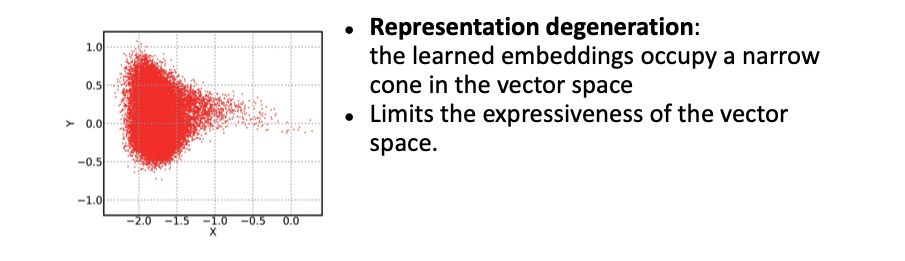
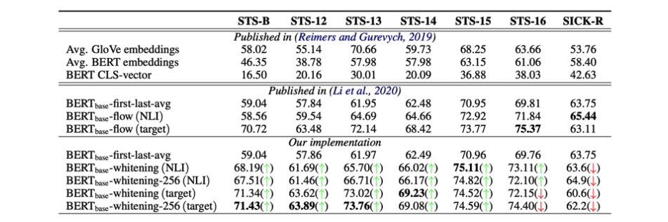
Diagram showing BERT’s sentence vectors forming a narrow, cone-shaped cluster concentrated in a small region of the embedding space, illustrating the anisotropy problem — Anisotropy problem in BERT’s representation space

Since the problem lies in the distribution, that’s where the fix comes from. BERT-flow tries to transform sentence embeddings from a Non-Smooth Anisotropic distribution into a Smooth Isotropic Gaussian one; BERT-whitening takes a simpler route, applying a whitening technique as post-processing to achieve a similarly more isotropic distribution. Both measurably improve the quality of BERT’s sentence representations.

Bar chart comparing scores of vanilla BERT, BERT-flow, and BERT-whitening on sentence similarity benchmarks — BERT-flow and BERT-whitening improve BERT’s performance on Sentence-Level Representation

9 #8: Using Contrastive Learning to Improve BERT’s Sentence Representations

Self-Supervised Learning (SSL) has been a wave over the past few years — the core idea is to design pretext tasks that let a model exploit large amounts of unlabeled data. BERT itself was trained this way, using two pretext tasks: Masked Language Modeling and Next Sentence Prediction.

SSL methods roughly split into Self-Prediction and Contrastive Learning; the two pretext tasks BERT uses fall into the first category. Contrastive Learning, meanwhile, has had a remarkable run in Computer Vision over the past few years, to the point where it can now beat supervised models on ImageNet classification.

If you’re not familiar with SSL, besides Hung-Yi Lee’s Self-supervised Learning course, this NeurIPS 2021 tutorial (given by Lilian Weng) is also a great reference. If you want a fast catch-up on Contrastive Learning’s progress in CV specifically, this video walks through 14 well-known papers in one go — I found it genuinely useful.

Back to the main topic. In this section, the speaker walks through a large number of papers that use Contrastive Learning to help BERT learn better sentence representations, grouped into seven categories:

Designed Positives
Generating Positives
Bootstrapping Methods
Dropout Augmentations
Equivariant Contrastive Learning
Prompting
Ranking-based Methods

Almost all seven categories are, underneath, answering the same question: where does the Positive Sample come from? Let’s go through them one at a time.

9.1 Designed Positives

The first category, Designed Positives, uses some hand-designed mechanism to pick Positive Samples out of existing data.

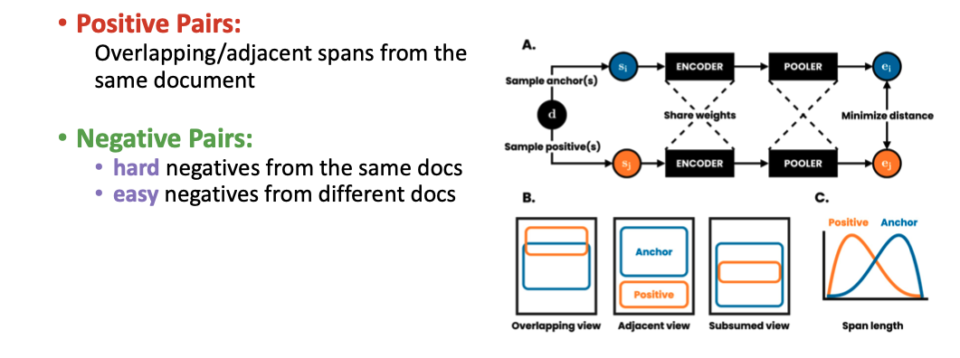
Diagram showing two overlapping or adjacent text spans within a document being labeled as a positive pair — DeCLUTR defines Positive Samples using overlapping or adjacent spans within a single document

DeCLUTR’s idea is intuitive: within the same document, if two spans overlap or are adjacent, they’re probably semantically close, so treat them as a Positive Sample.

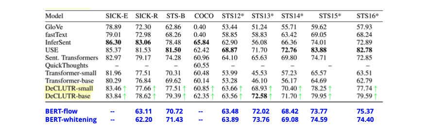
Bar chart comparing DeCLUTR’s scores against BERT-flow and BERT-whitening — DeCLUTR outperforms BERT-flow and BERT-whitening

As the figure shows, the Contrastive Learning-based approach beats the previous section’s BERT-flow and BERT-whitening.

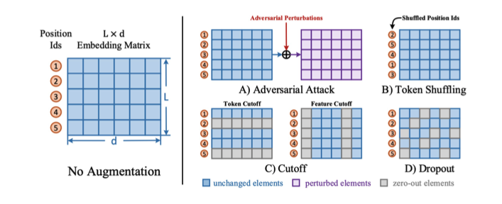
Flowchart showing multiple augmentation techniques applied at the token embedding space level to generate positive pairs — ConSERT applies various augmentations in the Token Embedding Space to generate Positive Samples for Contrastive Learning

ConSERT moves the manipulation elsewhere: instead of augmenting the raw text, it applies various augmentations directly to the Token Embedding Space to generate Positive Samples.

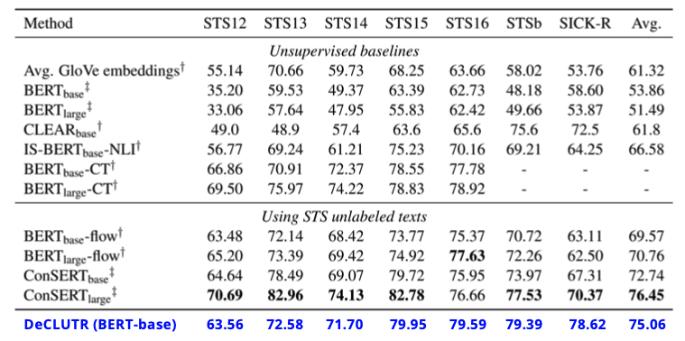
Bar chart comparing ConSERT’s scores against DeCLUTR — ConSERT outperforms DeCLUTR

The experimental numbers show ConSERT doing even better than DeCLUTR.

9.2 Generating Positives

The previous two methods “pick” or “modify” existing data to get Positive Samples. Generating Positives takes it further, generating a Positive Sample from scratch.

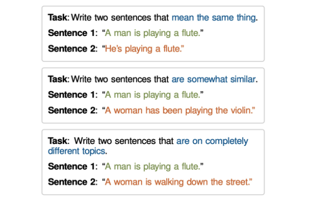
Flowchart showing GPT-2 used as a generator to produce a semantically similar sentence directly as a positive sample — DINO generates Positive Samples directly using GPT-2’s generative power

DINO is the representative of this route, using GPT-2’s generative ability to produce Positive Samples directly.

9.3 Bootstrapping Methods

In Contrastive Learning, the number of Negative Samples is often the deciding factor — too few, and the model can’t learn good representations. This is a practical headache too, since a large number of Negative Samples usually means a large batch size and heavy GPU memory pressure. But since Bootstrap Your Own Latent: A New Approach to Self-Supervised Learning (BYOL) was proposed, it’s become possible to do Contrastive Learning without any Negative Samples at all.

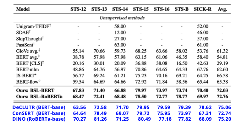
Bar chart comparing a BYOL-style sentence representation method against methods that include negative samples — Using BYOL to help BERT learn Sentence Representations (though it underperforms Contrastive Learning methods that include Negative Samples)

Bootstrapped unsupervised sentence representation learning is exactly this: applying BYOL’s idea to BERT’s Sentence Representation Learning. Unfortunately, per the results above, it still trails methods that do use Negative Samples (DeCLUTR, ConSERT, DINO).

9.4 Dropout Augmentations

The fourth category is Dropout Augmentations, whose flagship paper is the well-known SimCSE.

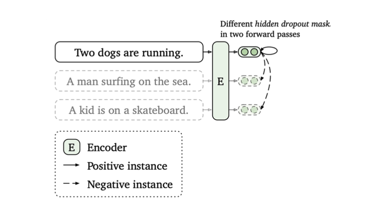
Diagram showing the same sentence passed through the same model twice, with different neurons masked out by dropout each time, producing two different embeddings — SimCSE uses dropout in place of directly augmenting the input

SimCSE’s approach is surprisingly simple: instead of augmenting the input at all, it applies dropout to the Transformer layers. The same sentence is fed through the same model twice, using the same dropout probability but dropping different neurons each time, so it comes out as two different embeddings. Since both come from the same sentence, they’re a natural Positive Sample.

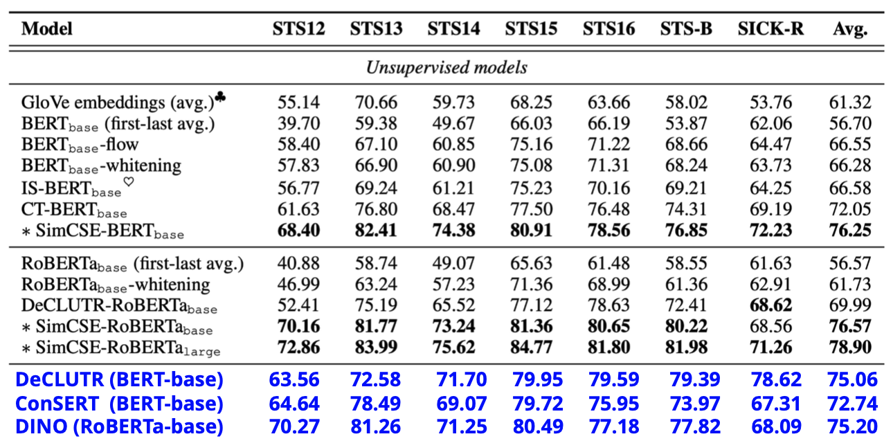
Bar chart comparing SimCSE against DeCLUTR, ConSERT, and DINO on a sentence similarity benchmark — SimCSE outperforms other augmentation-based approaches to generating Positive Samples

The results show that this “do nothing but dropout” approach outperforms the more elaborately designed augmentation methods — DeCLUTR, ConSERT, and DINO.

9.5 Equivariant Contrastive Learning

SimCSE’s result exposes something important: designing data augmentation for NLP is genuinely hard. Text is discrete — change one word and the meaning can shift entirely — so no matter how carefully an augmentation is designed, it still underperforms simply applying dropout to the model.

Thinking back, the point of using data augmentation to produce Positive Samples was to make the model’s representation Invariant to those augmentations. But looking at the progression from DeCLUTR, ConSERT, and DINO to SimCSE, that premise actually hurt performance in NLP.

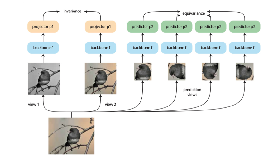
Two training objectives shown side by side, one requiring the representation to stay unchanged under augmentation, the other requiring it to reveal what augmentation was applied — Equivariant Contrastive Learning includes two kinds of tasks at once

That led to Equivariant Contrastive Learning: some methods aim to learn good representations through an Invariance Task (left side of the figure above), while others aim for it through an Equivariance Task (right side). Invariance means “however you change it, the representation stays the same”; Equivariance is the opposite — “the representation should reflect exactly what change you made.”

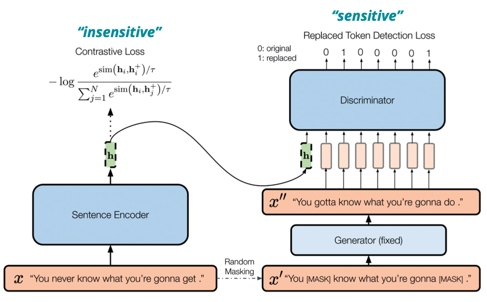
Architecture diagram of DiffCSE showing an invariance-task sentence encoder branch on the left and an equivariance-task discriminator branch on the right — DiffCSE trains a Sentence Encoder using both kinds of task, based on Equivariant Contrastive Learning

DiffCSE builds on Equivariant Contrastive Learning, training a Sentence Encoder with two tasks at once: the left half handles the Invariance Task, the right half the Equivariance Task. At inference time, only the left-half Sentence Encoder is actually used — the right half is purely a training-time aid.

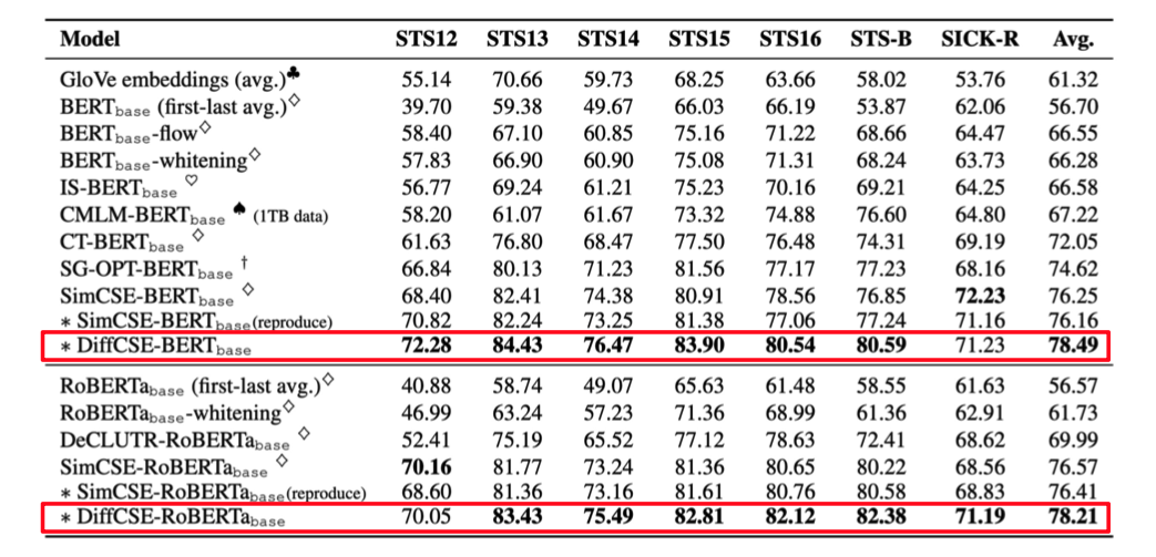
Bar chart comparing DiffCSE against SimCSE on sentence similarity benchmarks — DiffCSE outperforms SimCSE

The results show DiffCSE beating SimCSE by roughly 2–3%.

9.6 Prompting

The sixth category is Prompting, represented by PromptBERT: Improving BERT Sentence Embeddings with Prompts.

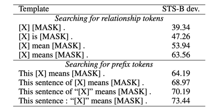
Diagram showing a sentence inserted into a prompt template with placeholders, with the hidden state at the mask position taken as the sentence vector — Learning sentence embeddings by designing a prompt template

PromptBERT designs a set of prompt templates, slots the sentence to be encoded into the template’s [X] position, feeds the whole prompt into BERT, and takes the hidden state at the [MASK] token as that sentence’s embedding. In effect, this lets BERT produce a sentence vector using the exact pose it’s most comfortable with — Masked Language Modeling — instead of forcing an average over a bunch of tokens.

9.7 Ranking-based Methods

The last category is Ranking-based Methods, represented by RankEncoder: Ranking-Enhanced Unsupervised Sentence Representation Learning. Its angle is that a sentence’s meaning can be described by its relative relationship to other sentences.

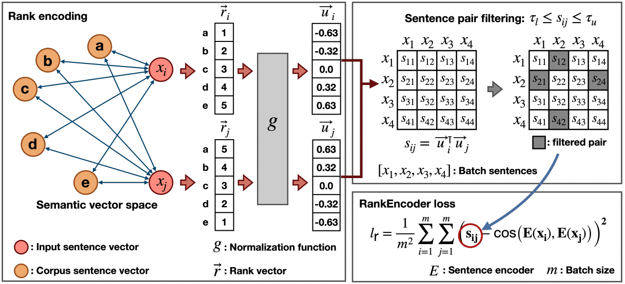
Flowchart showing two sentences each compared for similarity against an external corpus to form rank vectors, which are then combined by inner product to get their similarity — RankEncoder learns a sentence’s embedding using information about its neighbors

The specific method: given two sentences, compute each one’s similarity to every sentence in an external corpus, forming a Rank Vector for each. Normalize the two Rank Vectors and take their inner product, and that’s the similarity between the two sentences. The bottom-right of the figure above is the training objective: RankEncoder learns to convert the two sentences into representations whose cosine similarity approaches the similarity computed from “neighbor information.”

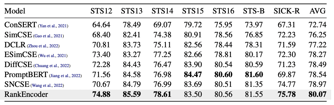
Summary table of scores comparing RankEncoder against all the previously discussed sentence representation methods — Sentence representations learned by RankEncoder reach SOTA

As the figure shows, RankEncoder beats nearly every method discussed so far.

10 #9: The Idea Behind Parameter-Efficient Fine-tuning

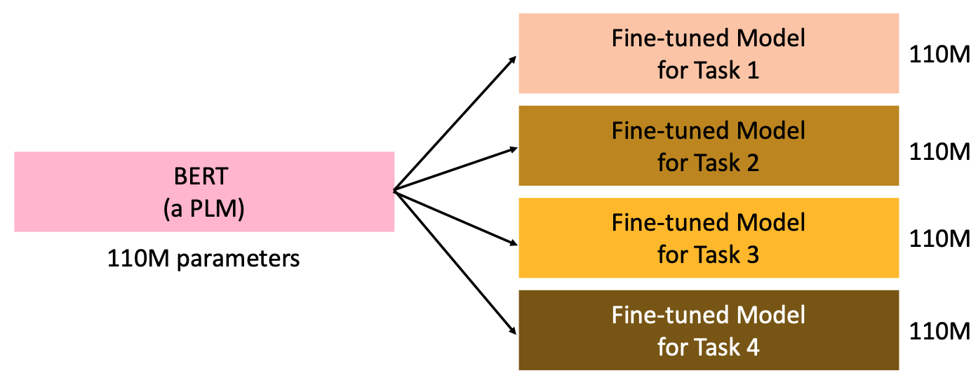
Diagram showing a full pre-trained model duplicated and independently trained into a separate copy for each of several downstream tasks — In the usual fine-tuning approach, the entire pre-trained model is trained on the downstream task

Once you have a pre-trained model, the standard move is to fine-tune it on a downstream task. The problem is that this “standard move” gets expensive fast: with 5 downstream tasks, you’d fine-tune the “whole” pre-trained model 5 times, ending up with 5 saved weight sets each nearly as large as the original model.

As pre-trained models keep getting bigger, this path stops being viable — most people simply don’t have the GPU memory to fine-tune an entire model. We need a way to fine-tune without touching that many parameters, and that family of methods is called Parameter-Efficient Fine-tuning (PEFT).

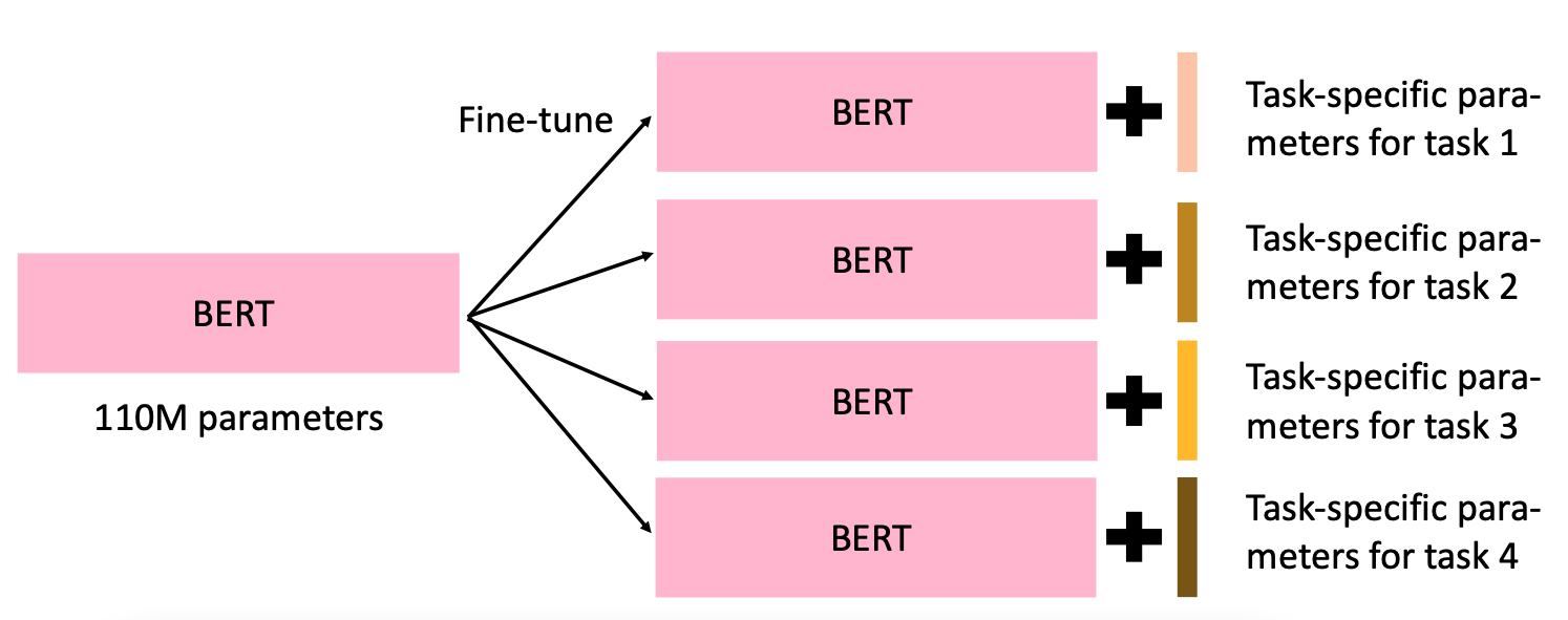
Architecture diagram showing the main body of a pre-trained model kept frozen, with a small module inserted and only that module trained — Parameter-Efficient Fine-tuning inserts a small extra module into the pre-trained model and only fine-tunes that module

PEFT works by inserting small extra modules into the pre-trained model and only training those modules during fine-tuning. That way, what needs to be saved for each downstream task is no longer a full copy of the large model — just the parameters of those extra modules.

So why does fine-tuning just a small slice of parameters even work? That comes back to what fine-tuning is fundamentally for: fine-tuning aims to change the pre-trained model’s representation so it performs better on the downstream task.

Conceptual diagram showing an original representation h becoming h-prime after fine-tuning, with the difference between them labeled delta-h — Fine-tuning aims to change the pre-trained model’s representation so it performs better on the downstream task

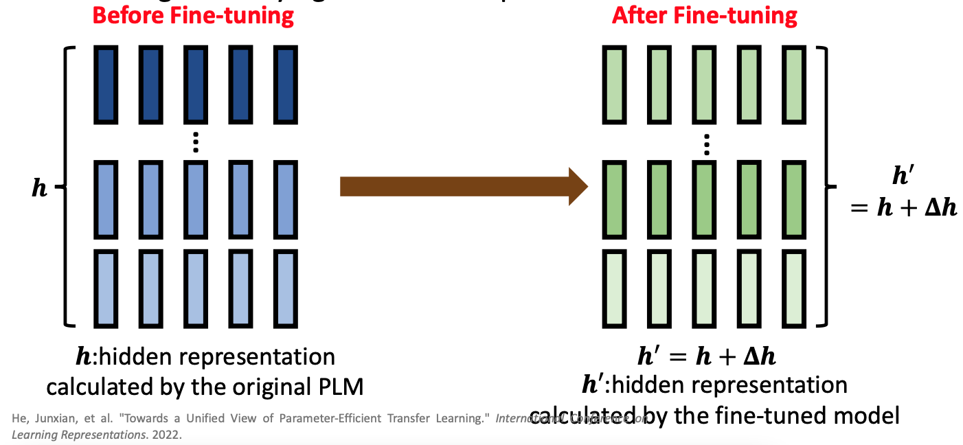
The figure above makes this concrete: the pre-trained model’s original representation is h; after fine-tuning the whole model, the representation becomes h_prime. If the only goal is to get from h to h_prime, why touch the whole model at all? PEFT’s core idea is to add a small module that produces an additional delta_h, such that h + delta_h = h_prime.

PEFT has four main implementations, covered one by one below:

Adapter
LoRA
Prefix Tuning
Soft Prompting

11 #10: PEFT — Adapter

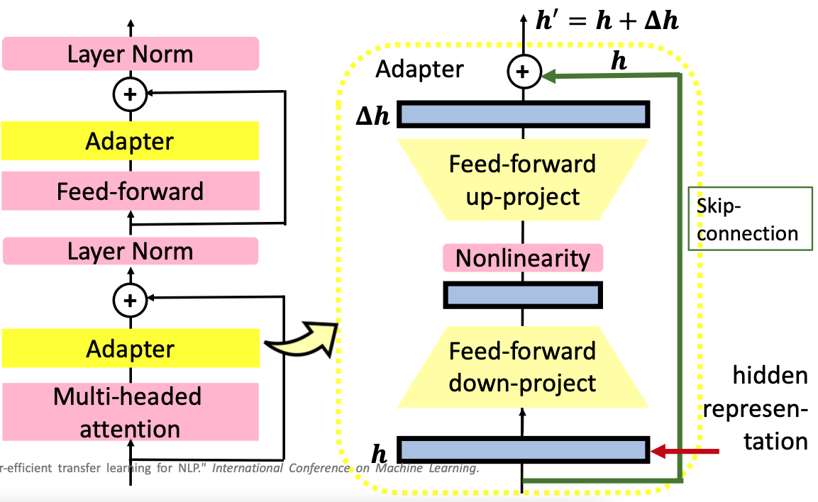
Diagram showing an Adapter module inserted after both self-attention and the feed-forward layer in a Transformer layer, with a zoomed-in view showing the adapter’s two feed-forward layers and skip connection — Adapter diagram

The idea behind Adapter is to insert a small extra module right after the Multi-Head Self-Attention block and again after the Feed-Forward Layer within a Transformer layer — this module is what’s called an Adapter. Its architecture is shown on the right of the figure above: two feed-forward layers sandwiching a non-linear layer, plus a skip connection.

Mapping this back to #9’s h and delta_h: the two feed-forward layers plus the non-linear layer are what transform the original representation h into delta_h, and the skip connection is what adds h and delta_h together to get the fine-tuned h_prime.

12 #11: PEFT — LoRA (Low-Rank Adaptation of Large Language Models)

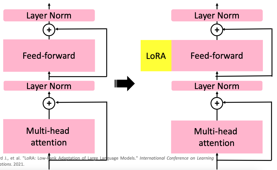
Overall architecture diagram showing an extra module attached in parallel next to the feed-forward layer of a Transformer layer — LoRA diagram

LoRA’s approach is to attach an extra module alongside the Feed-Forward Layer within a Transformer layer.

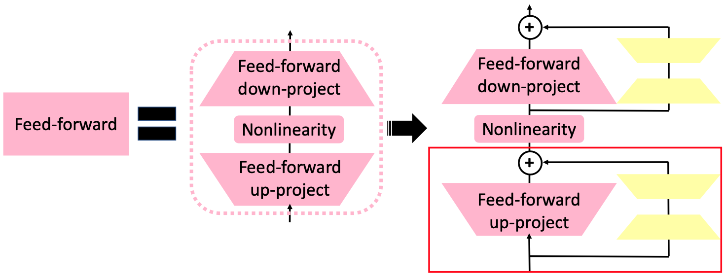
Diagram showing the two-layer structure of a feed-forward layer with a parallel branch, also made of two layers, attached beside it — LoRA adds a branch alongside the Transformer layer’s Feed-Forward Layer

Concretely, the Feed-Forward Layer inside a Transformer layer is actually made of two layers; LoRA adds a branch next to those two layers, and that branch is itself made of two layers as well.

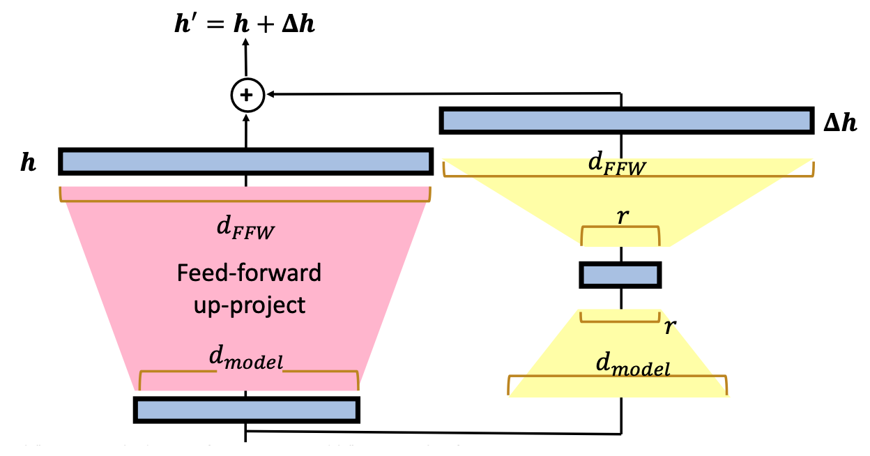
Diagram showing an input vector first projected down to a very small dimension and then projected back up, with the output added to the main branch — A LoRA module projects the original representation into a much smaller dimension before projecting it back up to produce a new representation

What’s distinctive is that a LoRA module first projects the original input down into a very small dimension, then back up to produce a new representation (delta_h), which is finally added to the original representation (h) to get h_prime. This “squeeze then expand” is exactly what “low-rank” means, and it’s also why LoRA’s parameter count stays so small.

13 #12: PEFT — Prefix Tuning

Literally, a prefix is something attached to the “front” of something else, and Prefix Tuning is fine-tuning only that thing attached to the front.

To understand how it works, we need a quick refresher on Self-Attention.

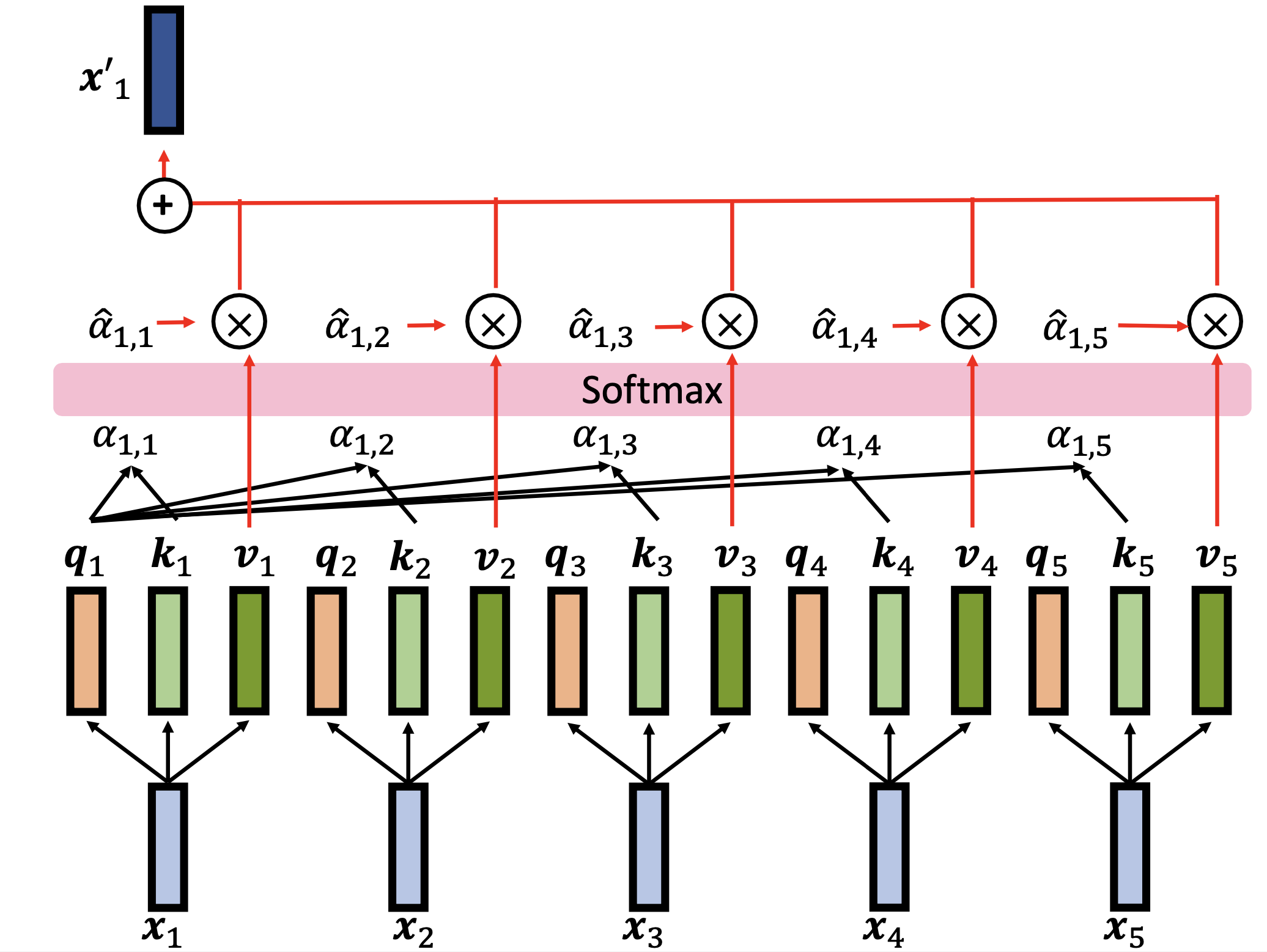
Flowchart showing each vector in a sequence going through query, key, and value projections, then computing a weighted sum over all values using attention scores — How Self-Attention works

The figure above shows Self-Attention’s mechanics: every vector in a sequence gets its own Query, Key, and Value through a set of Query, Key, and Value Projections. When computing x1’s output, we take x1’s Query and match it against the Key of every vector (including itself) to get an Attention Score, which represents how relevant x1 is to each vector. That Attention Score is then used to compute a weighted sum over every vector’s Value — that weighted sum is x1’s output.

In Prefix Tuning, we add some extra vectors to the “front” of the input to the Self-Attention layer, and those vectors are called the Prefix.

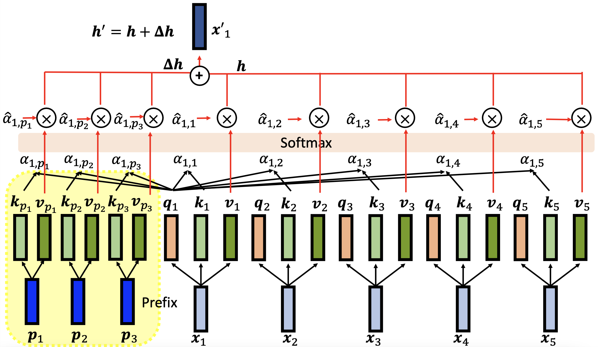
Diagram showing several additional vectors inserted before the input sequence to a self-attention layer, participating in the same attention computation as the rest of the sequence — Prefix Tuning adds extra vectors to the front of the Self-Attention layer’s input sequence

As shown above, once the Prefix is added, computing x1’s output now also has to factor in the Prefix’s Query, Key, and Value. The weighted sum over the original vectors’ Values gives the original representation (h), and the weighted sum over the Prefix’s Values gives delta_h; adding the two together gives the fine-tuned h_prime. Same h + delta_h pattern as before — this time, delta_h just comes from within attention itself.

14 #13: PEFT — Soft Prompting

Adapter, LoRA, and Prefix Tuning are the three most common PEFT techniques; the fourth — and most often overlooked — is Soft Prompting.

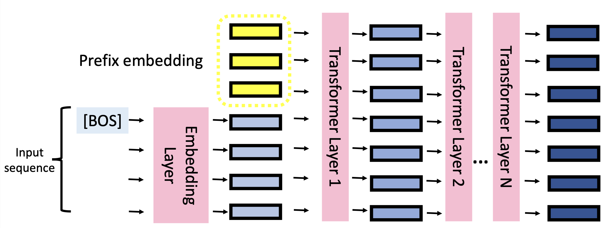
Diagram showing several trainable prefix embeddings attached in front of the embeddings produced by the embedding layer, before being fed into the transformer — Soft Prompting adds trainable Prefix Embeddings to the output of the Embedding Layer

Soft Prompting works even further upstream: the original input sequence passes through the Embedding Layer to produce a series of embeddings (the blue part in the figure above), and we attach some extra Prefix Embeddings before feeding everything into the transformer together. These Prefix Embeddings are trainable vectors that don’t need to correspond to any real word.

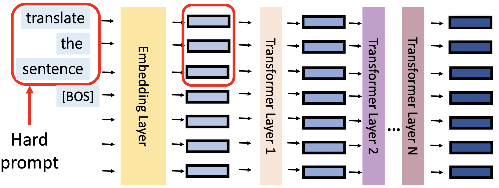
Diagram showing actual words added directly in front of the raw input text before it is fed into the embedding layer, contrasted with soft prompting — Hard Prompting instead adds real words directly into the input sequence

The opposite of Soft Prompting is Hard Prompting — the kind of prompting most people already know, where you add extra words directly into the original input sequence. The difference is that Hard Prompting adds words a human can read, while Soft Prompting adds vectors the model has learned on its own that a human can’t interpret.

15 Conclusion

These notes cover some of the ideas I found most worth remembering from the AACL-IJCNLP 2022 Tutorial: Recent Advances in Pre-trained Language Models — from what a PLM actually learns, to why sentence representations are hard, to the four mainstream PEFT approaches.

Looking back, the PEFT line of work has become especially important in the years since — LoRA has all but become the default choice for fine-tuning large models. Most of the illustrations in this post are taken from the tutorial itself; for the full picture, I’d recommend watching the video or reading the slides directly.