Understanding Backpropagation: How Gradients Are Calculated

Hong-Wei Wu included in category Essential AI Concept

2026-07-15 2026-08-02 3018 words 14 minutes

How are the gradients in a neural network actually computed? This article defines the notation, then walks through all four backpropagation equations, BP(1) to BP(4).

Contents

1 Introduction

In previous articles, we already learned that the parameters of a neural network can be updated using Gradient Descent and Stochastic Gradient Descent. At that point, however, we only described things conceptually — “adjust the weights and biases in the direction opposite to the gradient” — and never explained how those gradients are actually computed.

This article fills that gap: how the backpropagation algorithm computes the gradients of every parameter in a neural network in one go. We will start from the notation, then introduce the four core equations of backpropagation, and explain how each of them is derived.

Key Takeaways (TL;DR)

Backpropagation is an algorithm for computing gradients quickly — its whole purpose is to work out $\partial C / \partial w$ and $\partial C / \partial b$ efficiently.
The four equations split into two groups: BP(1) and BP(2) compute each neuron’s error $\delta$ , while BP(3) and BP(4) turn $\delta$ into the gradients we actually want.
$\delta \equiv \partial C / \partial z$ represents a neuron’s current error: a large $\delta$ means the neuron’s weights and biases still need adjusting, while a $\delta$ close to 0 means they no longer do.
The whole derivation relies on a single tool from calculus: the chain rule.

Info

If you are not yet familiar with how a neural network updates its parameters, you may want to read these first:

2 What Is Backpropagation?

Backpropagation is an algorithm for computing gradients quickly. Why do we need it? Modern neural networks casually contain tens of millions of parameters, and every time we update a parameter we must first compute its gradient (the partial derivative of the cost function with respect to that parameter). Without an efficient way to compute all of those millions of gradients, training time would stretch out to something completely impractical, and deep learning would be off the table entirely.

The backpropagation algorithm appeared as early as the 1970s, but it only received serious attention after David Rumelhart, Geoffrey Hinton, Ronald Williams and others jointly published the 1986 paper Learning representations by back-propagating errors. That paper showed how backpropagation lets a neural network learn much faster, and from then on turned neural networks into a tool that could genuinely be used to solve problems.

To be honest, backpropagation is not an easy concept to digest. First-time readers easily get lost in the pile of mathematical symbols and subscripts. It is perfectly normal not to understand it on the first pass — it becomes clearer as you work through it a few more times.

Before drowning in notation, hold on to one guiding principle: backpropagation is an algorithm for computing gradients quickly — that is, for quickly computing $\partial C / \partial w$ and $\partial C / \partial b$ . With $\partial C / \partial w$ and $\partial C / \partial b$ in hand, we know whether the cost function’s value will increase or decrease when a weight (w) or bias (b) changes, and by how much. Every derivation in this article ultimately exists to answer that question.

3 Computing a Neural Network’s Output

Before getting into backpropagation, make sure you understand how a neural network’s output is computed, and let’s pin down all the mathematical notation we will need later. If this section’s notation isn’t established first, the equations that follow will be very hard to read.

3.1 Defining the notation: w, b and a

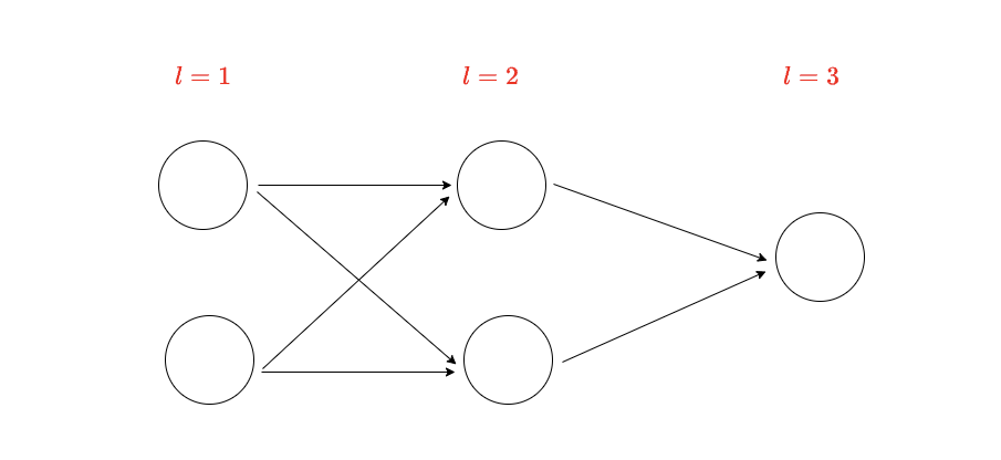
Diagram of a three-layer neural network made up of an input layer, a hidden layer and an output layer — A neural network with 3 layers

As shown above, this is a neural network with 3 layers, and we use a lowercase “L” to indicate which layer we are referring to.

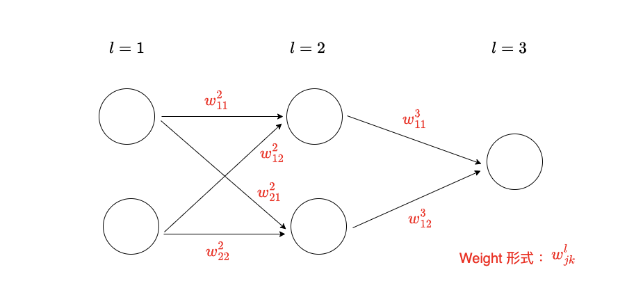
Neural network diagram highlighting the weight symbol w on a connection between two neurons, along with the meaning of its superscript and subscripts — Using w to denote the weights in a neural network

We use w to denote the weights in a neural network. Its form is the weight connecting the k-th neuron in layer L – 1 to the j-th neuron in layer L. The order of the subscripts (j first, then k) is easy to get backwards, so feel free to come back to this figure when reading the equations later.

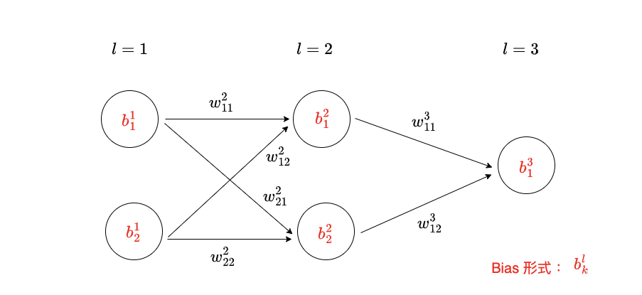
Neural network diagram highlighting each neuron’s own bias symbol b, along with the meaning of its superscript and subscript — Using b to denote the biases in a neural network

We use b to denote the biases in a neural network. Its form refers to the bias of the k-th neuron in layer L.

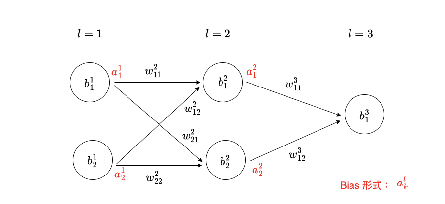
Neural network diagram highlighting each neuron’s output activation symbol a, along with the meaning of its superscript and subscript — Using a to denote the activations of a neural network

We use a to denote the activations in a neural network. Its form is the same as that of the bias — it refers to the k-th neuron in layer L.

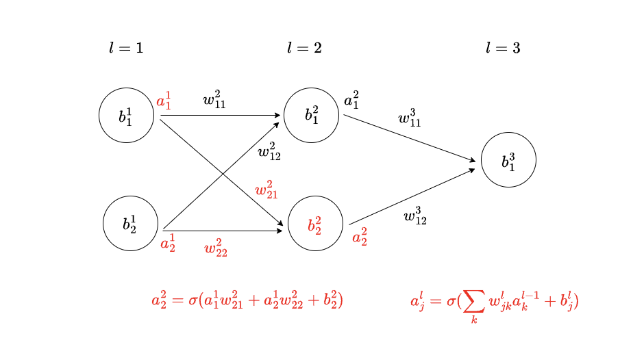
The activation equation: the weighted sum of the previous layer’s activations plus a bias, passed through a sigmoid function — Computing the activations in a neural network

The activation is computed as shown above: the weighted sum of the previous layer’s activations plus the bias, finally passed through an activation function (here we use the sigmoid function; for details, see the article An Improved Perceptron: Understanding the Sigmoid Neuron).

3.2 Simplifying with matrices and vectors

Writing this out neuron by neuron gets very tedious, so we use matrices and vectors to package up an entire layer’s information. For example, we use $w^l$ for all the weights in layer L, where $w^l_{jk}$ is the element in row j, column k of $w^l$ ; $b^l$ for all the biases in layer L; and $a^l$ for all the activations in layer L. In matrix and vector form, we can express the activation computation like this:

The activation equation written in vector and matrix form — Expressing the activation computation with vectors and matrices

Written this way it is much clearer: this layer’s activations are simply the previous layer’s activations multiplied by the weights, plus the bias, and finally passed through the sigmoid function. An entire layer’s computation collapses into a single line.

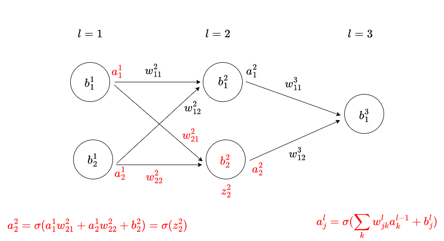
To make what follows easier, let’s define one more symbol. We define the content inside the sigmoid function in the activation equation above as z — in other words, $z^l \equiv w^l a^{l-1} + b^l$ . We can think of $z^l$ as the weighted input of the neurons in layer L, that is, the value before it passes through the activation function. With $z^l$ , the activation computation simplifies further to $a^l = \sigma(z^l)$ (as shown below).

Equation defining z as a neuron’s weighted input and simplifying the activation to σ(z) — Using z to denote a neuron’s weighted input

4 The Four Key Equations of Backpropagation

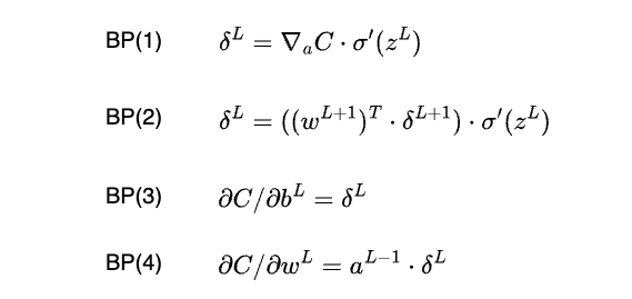
At this point the warm-up is complete (hopefully your head is still clear). Recall that the goal of the backpropagation algorithm is to quickly compute the gradient of every parameter in a neural network (the partial derivative of the cost function with respect to that parameter). This is accomplished mainly through the following four equations — every single $\partial C / \partial w$ and $\partial C / \partial b$ comes out of these four expressions:

The four backpropagation equations BP(1) through BP(4) presented side by side in one figure — The four key equations of the backpropagation algorithm

4.1 An intuitive first look at the four equations

Don’t panic — you certainly can’t read these four equations yet, and that is entirely normal. Before taking them apart one by one, let’s just observe their shape intuitively.

BP(3) and BP(4) both compute the partial derivative of the cost function with respect to the network’s parameters (weights and biases) — isn’t that exactly the gradient we want? And both of them involve $\delta$ . Looking back at BP(1) and BP(2), you’ll notice that both of those equations are computing $\delta$ .

In other words, the four equations really split into two groups: the first two compute $\delta$ , and the last two convert $\delta$ into the gradients we want. So what exactly is $\delta$ ? Before dissecting BP(1) through BP(4), let’s understand what $\delta$ means.

4.2 What δ means: the little sprite living inside a neuron

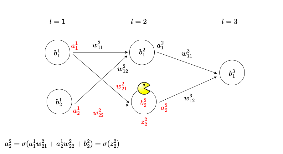
Neural network diagram with a little sprite drawn on the second neuron of the second layer — Imagine a little sprite living inside the neural network

Imagine that a little sprite lives inside the neural network. As shown above, the sprite lives in the second neuron of the second layer.

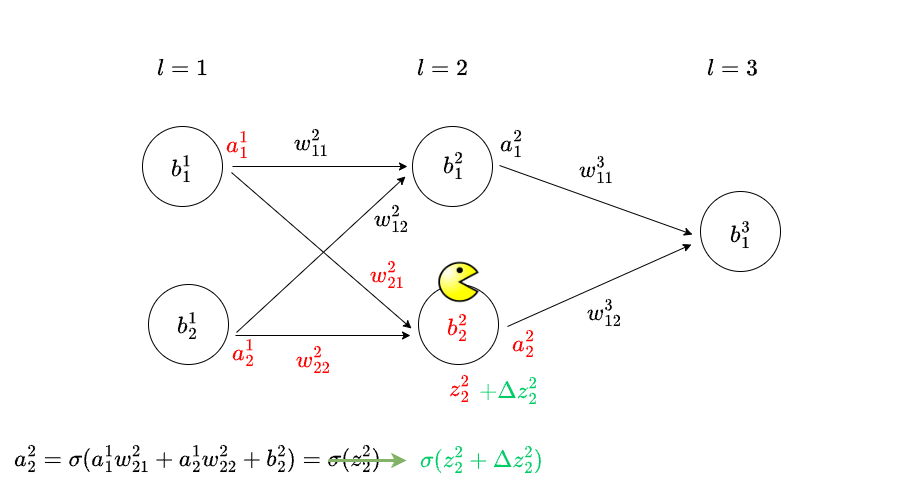
Diagram showing the sprite adding Δz to a neuron’s weighted input, changing the output from σ(z) to σ(z + Δz) — The mischievous sprite tampers with a neuron’s input

This sprite is very mischievous and tampers with this neuron’s input, so that the neuron’s final output (activation) changes from $\sigma(z)$ to $\sigma(z + \Delta z)$ . Because this neuron’s output changed, the outputs of the neurons after it change too, all the way through to the final value of the cost function. The change in the cost function is the gradient of z multiplied by the change in z, i.e. $\partial C / \partial z \times \Delta z$ .

Fortunately, although mischievous, this sprite is good-natured: it wants to add just the right amount of tampering ( $\Delta z$ ) to make the cost function’s value as small as possible. If $\partial C / \partial z$ is positive, it means C increases as z increases, so the sprite makes $\Delta z$ negative; if $\partial C / \partial z$ is negative, it means C decreases as z increases, so the sprite makes $\Delta z$ positive. Put simply, as long as the sprite makes the sign of $\Delta z$ opposite to that of $\partial C / \partial z$ , the cost function’s value goes down. And if $\partial C / \partial z$ is already close to 0, the sprite no longer needs to tamper with this neuron’s input at all.

Think about it: how does the sprite tamper with a neuron’s input? By adjusting that neuron’s weights and biases, of course! So when $\partial C / \partial z$ approaches 0, it means there is no need to change this neuron’s weights and biases any further — which is to say, this neuron’s weights and biases are already in great shape.

That’s why we use $\delta$ to denote $\partial C / \partial z$ , representing this neuron’s current error: if $\delta$ is large (in either the positive or the negative direction), this neuron’s weights and biases still need adjusting; conversely, if $\delta$ approaches 0, this neuron’s weights and biases no longer need to be adjusted.

Looking at the four equations again with the meaning of $\delta$ in mind, you’ll find that they all revolve around $\delta$ : first compute each neuron’s error, then use that error to compute the partial derivatives of the cost with respect to the weights and biases, and finally decide how the parameters should be updated.

If everything so far still makes sense, then the groundwork is done. Let’s start with equation number one.

5 Backpropagation Equation 1 (BP 1)

The first equation of the backpropagation algorithm is:

Backpropagation equation BP(1), which computes the error δ of a neuron in the output layer — Backpropagation equation 1

BP(1) is used to compute the error of the neurons in the final layer (the output layer) of a neural network. This is where the entire chain of derivations begins: only once the last layer’s error has been computed is there anything to propagate backwards.

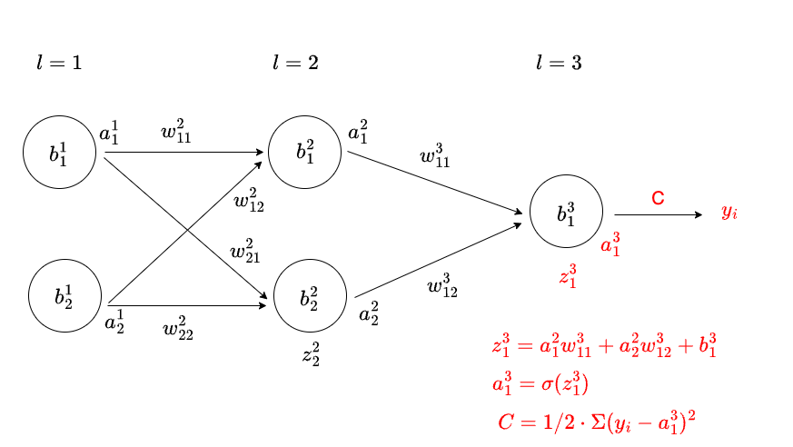
Equations showing the relationship between z, a and C for a neuron in the output layer — Computing z (weighted input), a (activation) and C (cost function) for a neuron in the output layer

The figure above shows how the weighted input (z) and activation (a) are computed for the first (and only) neuron in the output layer. Because this is an output-layer neuron, its output can be compared directly against the correct answer to compute the current cost.

We already know that $\delta$ (the left-hand side of BP(1)) is $\partial C / \partial z$ . The problem is that z doesn’t appear in the expression for C (because z is wrapped inside a), so we can’t take the partial derivative with respect to z directly. This is where calculus’s chain rule comes in: “the partial derivative of C with respect to z” equals “the partial derivative of C with respect to a” multiplied by “the partial derivative of a with respect to z”.

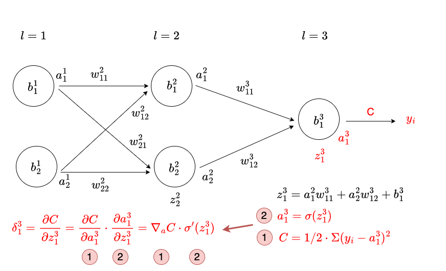
Derivation expanding ∂C/∂z into ∂C/∂a multiplied by ∂a/∂z via the chain rule — Using the chain rule to compute the partial derivative of C with respect to z

With that, where the first equation comes from is clear. BP(1) lets us compute the error of the neurons in a neural network’s output layer.

6 Backpropagation Equation 2 (BP 2)

The second equation of the backpropagation algorithm is:

Backpropagation equation BP(2), which derives the error of the previous layer’s neurons from the error of the next layer — Backpropagation equation 2

From BP(1) we already know how to compute the error of the output layer’s neurons; BP(2) then computes the error of the previous layer’s neurons based on the error of the current layer’s neurons. With BP(1) and BP(2) together, we can work backwards like a row of dominoes from the last layer all the way to the front, computing the error of every neuron in the network. This is exactly where the name backpropagation (backwards propagation of errors) comes from.

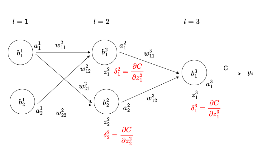
Diagram with an arrow pointing from the error at L=3 back to the error at L=2, showing errors propagating backwards — Using BP(2), we can derive the error at L=2 from the error at L=3

As shown above, BP(1) has already given us the error at L=3, and BP(2) explains how to work backwards from the L=3 error to the L=2 error.

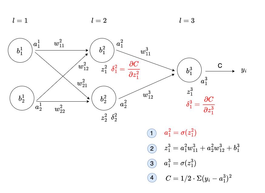
Four numbered equations ① to ④ showing how the z of the first neuron in the second layer connects through to the cost — The relationship between z and the cost for the first neuron in the second layer

The second layer (L = 2) has two neurons; let’s focus on the first one and work out how its error is computed. The four equations above (① ~ ④) show the relationship between this neuron’s z and the cost function (② ~ ④ were already introduced in BP(1)).

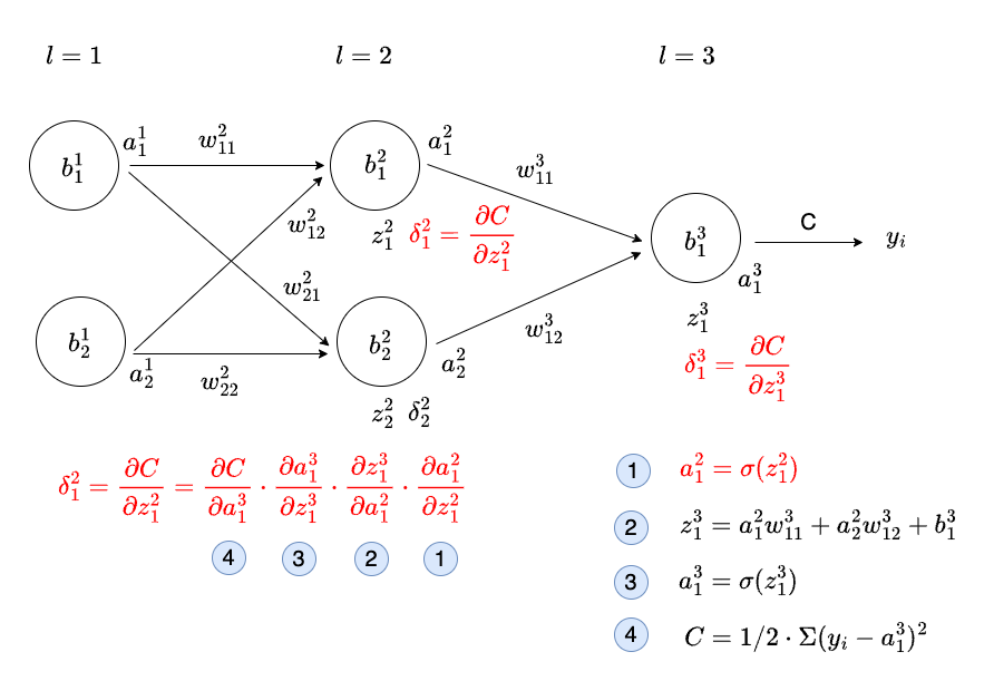
Derivation expanding the partial derivative of the cost with respect to a hidden-layer neuron’s z into a product of partial derivatives via the chain rule — Using the chain rule to compute the partial derivative of the cost with respect to a hidden-layer neuron’s z

Just as in BP(1), the cost function cannot take a partial derivative with respect to this neuron’s z directly, so once again we need the chain rule to help (as shown above).

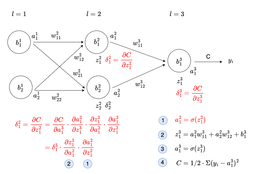
Rewritten equation substituting the product of ③ and ④ with the result already obtained in BP(1) — We already computed the product of ③ and ④ back in BP(1)

And because we already computed the product of ③ and ④ back in BP(1), we can substitute it straight in and rewrite the expression as shown above. This is also the key to why backpropagation is fast: results computed for the later layers don’t need to be recomputed — they are simply reused.

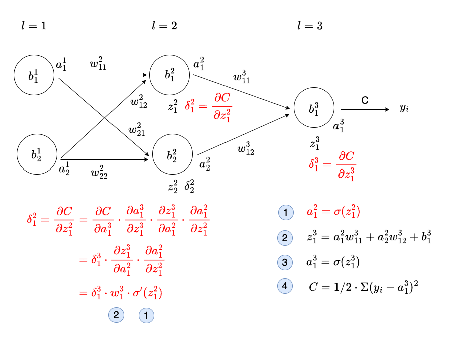
Derivation computing the partial derivatives of the two numbered equations ① and ② — Computing the partial derivatives of ① and ②

The remaining terms ① and ② are very simple expressions whose partial derivatives can be computed directly. With that done, let’s look back at backpropagation’s second equation:

The derivation is in fact already complete, but you may feel it doesn’t quite line up with the figure. That’s because the equation in the figure is expressed in matrix and vector form, whereas we just expanded things for a single neuron; the underlying arithmetic is exactly the same. BP(2) lets us compute the error of the neurons in a neural network’s hidden layers.

In other words, BP(1) and BP(2) together let us compute the error of every neuron in every layer of the network. BP(3) and BP(4), which come next, use those errors to compute what we actually want: $\partial C / \partial w$ and $\partial C / \partial b$ .

7 Backpropagation Equation 3 (BP 3)

The third equation of the backpropagation algorithm is:

Backpropagation equation BP(3): the partial derivative of the cost with respect to a bias equals that neuron’s error δ — Backpropagation equation 3

BP(3) states that the partial derivative of the cost function with respect to a bias is simply that neuron’s error. No multiplication needed — they are just equal. Why does it come out so clean?

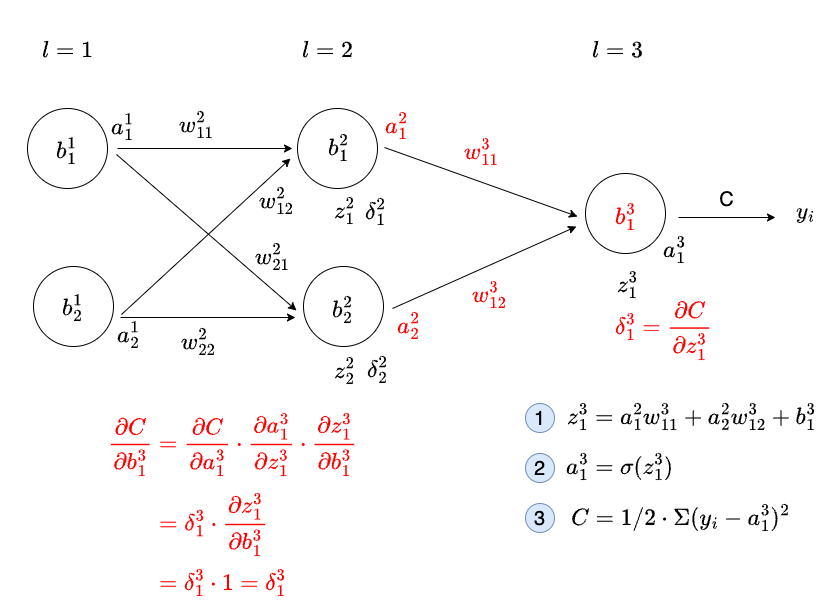
Numbered equations ① to ③ deriving the partial derivative of the cost with respect to a bias via the chain rule — Using the chain rule to compute the partial derivative of the cost with respect to a bias

As shown above, equations ① ~ ③ present the relationship between the bias of the first neuron in the output layer and the cost. As with BP(2), C cannot take a partial derivative with respect to that bias directly, so we use the chain rule. Once expanded, we find that the partial derivative of z with respect to b happens to be 1, and the whole expression collapses to $\partial C / \partial b$ simply being $\delta$ .

BP(3) lets us compute the partial derivative of the cost function with respect to every bias in the neural network, and hence which direction each bias should be updated in.

8 Backpropagation Equation 4 (BP 4)

The fourth equation of the backpropagation algorithm is:

Backpropagation equation BP(4): the partial derivative of the cost with respect to a weight equals the previous layer’s activation multiplied by that neuron’s error — Backpropagation equation 4

Finally we arrive at the last equation. BP(4) states that the partial derivative of the cost function with respect to a weight is that neuron’s error multiplied by “the incoming activation”.

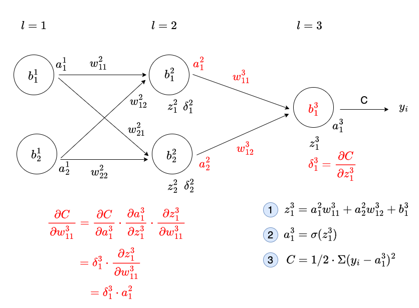
Numbered equations ① to ③ deriving the partial derivative of the cost with respect to a weight via the chain rule — Using the chain rule to compute the partial derivative of the cost with respect to a weight

As shown above, equations ① ~ ③ present the relationship between the first weight of the first neuron in the output layer and the cost. Because C cannot take a partial derivative with respect to that weight directly, we again use the chain rule. You’ll notice the whole process is basically identical to BP(3); the only difference is that the final differentiation yields not 1, but the previous layer’s activation.

BP(4) lets us compute the partial derivative of the cost function with respect to every weight in the neural network, and hence how each weight should be updated.

9 Conclusion

That covers the principles behind the backpropagation algorithm. The whole procedure boils down to two sentences: first use BP(1) to compute the output layer’s error, then use BP(2) to propagate that error backwards layer by layer; with every neuron’s error in hand, BP(3) and BP(4) directly convert them into the partial derivatives of the cost with respect to every bias and weight, which are then handed to Gradient Descent to update the parameters.

If you’ve read this far, taking one more look at this figure should be enough for you to read the meaning of every equation in it:

And if there are still parts you don’t understand, don’t be discouraged. The very fact that you’re willing to dig into how a neural network updates itself already puts you ahead of many people who “learn AI by calling libraries”. This topic simply takes a few passes to fully digest — come back to it in a few days and it will feel very different.