Probability From Zero: Marginal, Joint & Conditional

1 Introduction

Probability is the foundation of machine learning. Whether it’s Naive Bayes, a language model computing the distribution over the next token, or evaluating how confident a model’s output is, they’re all speaking the same underlying language of probability. Without a solid foundation, every formula you see later just becomes something to memorize.

The problem is, most probability tutorials online assume you already have some background — they open with a string of symbols, and beginners get stuck within the first paragraph. This article assumes you have zero background in probability. It starts from the most basic idea, “notation,” then walks through the three most common types of probability — marginal, joint, and conditional — and finally ties all three together with the multiplication rule.

2 Probability Notation

The concept of probability is always tied to some “event.” An event here isn’t anything mysterious — it’s just a description of something that happens. “Today is rainy,” “rolling a die and getting a 3,” “drawing a red ball from a bag” — these are all events.

We use probability to describe how likely an event is to happen. Using the examples above, we might say “the probability that today is rainy is 50%,” “the probability of rolling a 3 is 1/6,” or “the probability of drawing a red ball is 30%.”

An event usually has more than one possible outcome, and each outcome has some chance of happening. The reason we need probability to describe it in the first place is that we don’t know in advance which outcome will occur — the outcome itself is random. In mathematics, the variable that describes all the possible outcomes of an event is called a random variable.

Take rolling a die as an example. The result can be 1, 2, 3, 4, 5, or 6, but nobody knows which one it’ll be before the roll. Mathematically, we define a random variable $X = \{1, 2, 3, 4, 5, 6\}$ to represent all possible outcomes of the roll.

In words, the same idea reads like this:

• The result of the die roll is one of 1, 2, 3, 4, 5, 6
• The probability that the result of the die roll is 1

In math, it’s written like this:

• $X = \{1, 2, 3, 4, 5, 6\}$
• $P(X=1)$

Comparing the two makes it clear: the random variable $X$ describes all the possible outcomes of an event, while $P(X=1)$ describes the probability of one specific outcome (P is shorthand for Probability). Every formula that follows is built on these two symbols, so getting comfortable with them first will make everything else much easier.

3 Three Basic Types of Probability

With the random variable and the $P(...)$ notation in hand, let’s look at the three most basic types of probability: marginal probability, joint probability, and conditional probability.

All three use the same deck of playing cards as an example, which makes the differences easier to see. A standard deck has 52 cards, of which 4 are the number 6, and 26 are red.

• Marginal Probability Describes the probability of “one” event happening on its own. If A is an event, then $P(A)$ is a marginal probability. With the deck of cards, suppose A = “drawing a 6 from a deck of playing cards.” Then $P(A) = 4/52$ (there are 4 cards showing a 6 out of 52).

• Joint Probability Describes the probability of “two or more” events happening at the same time. If A and B are two different events, the probability of both happening at once is written $P(A \cap B)$. The “∩” symbol means “intersection” — in plain terms, “both conditions must hold.” With the deck of cards, suppose A = “drawing a 6” and B = “drawing a red card.” Then $P(A \cap B) = 2/52$ (out of 52 cards, only 2 are both a 6 and red).

• Conditional Probability Describes the probability of one event happening given that another event has already happened, written $P(A \mid B)$ and read as “the probability of A given B.” With the deck of cards, let B = “drawing a red card” and A = “drawing a 4.” Then $P(A \mid B) = 2/26$. The key is that the denominator changes: since we already know the card drawn is red, the scope shrinks from 52 cards down to the 26 red cards, and among those 26, there are 2 fours.

Here’s an easy way to remember the difference: marginal looks at a single event, joint requires multiple events to hold at the same time, and conditional first narrows the scope down to a known condition before looking at the probability of an event.

4 Tying the Three Together: The Multiplication Rule

Now that we’ve covered the three types of probability individually, let’s look at how they relate to each other — the multiplication rule.

The value of the multiplication rule is that it brings all three types of probability together into a single equation. A Venn diagram makes it even more intuitive.

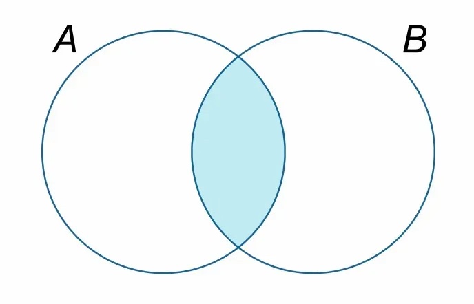
$P(B)$ is the probability of event B, corresponding to circle B in the diagram; $P(A)$ is the probability of event A, corresponding to circle A. $P(A \cap B)$ is the probability of A and B happening at the same time, corresponding to the overlapping region of the two circles.

So the probability of A happening given that B has already happened, $P(A \mid B)$, is “the probability of A and B happening together, $P(A \cap B)$,” divided by “the probability of B happening, $P(B)$.” Intuitively: once we know B has happened, the entire world shrinks down to circle B, and the only part of A that can still happen is the overlapping region — so we divide the overlapping region by circle B.

Verifying this with the playing-card example again makes it click. A = “drawing a 4,” B = “drawing a red card.” $P(A \cap B) = 2/52$ and $P(B) = 26/52$, so dividing them gives $(2/52) \div (26/52) = 2/26$ — matching the answer we got earlier by directly counting the red cards.

5 Conclusion

This article started from the most fundamental concepts — probability, event, and random variable — and then introduced three basic types of probability:

• Marginal probability: the probability of a single event happening
• Joint probability: the probability of multiple events happening at once
• Conditional probability: the probability of an event happening given some known condition

Finally, we tied all three together with the multiplication rule:

The follow-up article, Conditional vs Joint Probability: A Deck of Cards Clears It Up, covers more foundational concepts, going into more detail on the difference between joint probability and conditional probability, as well as the concepts of AND and OR in probability.