Machine Learning Basics: The Bias-Variance Tradeoff

1 Introduction
After a model has been trained, we measure its performance on a test dataset — that is, we compute the model’s error. That error is actually made up of two parts: bias and variance. Ideally we would like both to be as small as possible, but reality doesn’t allow it: reducing bias tends to raise variance, and conversely pushing variance down pulls bias up.
This article explains what a model’s bias and variance are, why the two pull against each other, and how far a model should be trained to strike a balance.
Before reading, it helps to have a basic grasp of “what machine learning is”, “models, training and inference in machine learning”, and “the five steps of machine learning” (all covered in earlier articles in this series).
- Bias is the error between a model’s output and the correct answer. High bias means the model hasn’t learned the relationship between input and output — that’s underfitting.
- Variance is how much a model’s output varies across different inputs. High variance means the model has memorised even the noise in the training data — that’s overfitting.
- The two move in opposite directions as model complexity changes, so they cannot both be minimised at once.
- What you should actually aim for is not driving either one to its minimum, but landing total error at the bottom of the U-shaped curve.
2 A Model’s Bias
Once we have a training dataset, we start training the model on it. Training, put plainly, means repeatedly adjusting the parameters inside the model so that when data is fed in, the model’s output is as close to the correct answer (the label) as possible. Looked at another way, a model is just a function responsible for mapping input data to some output.
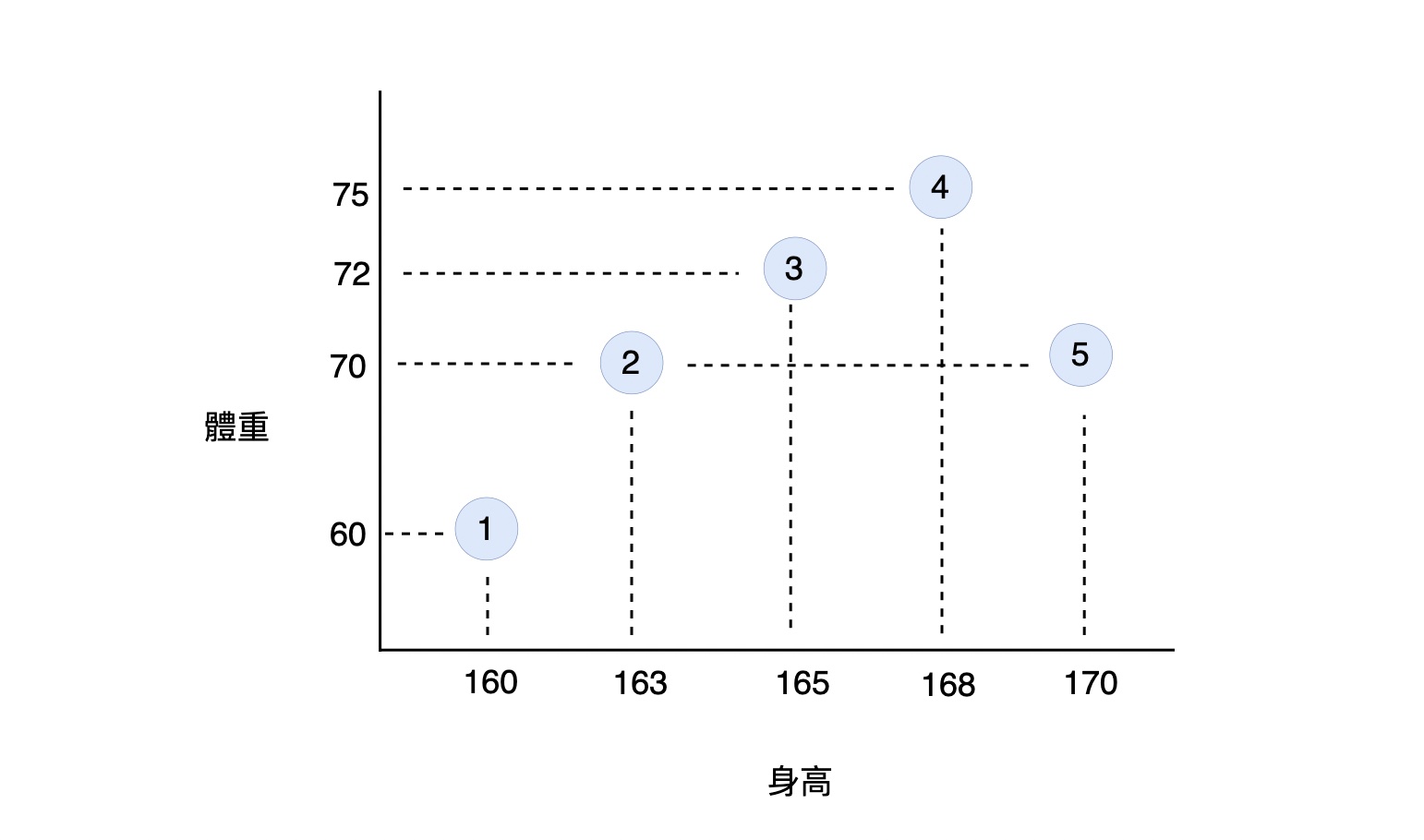
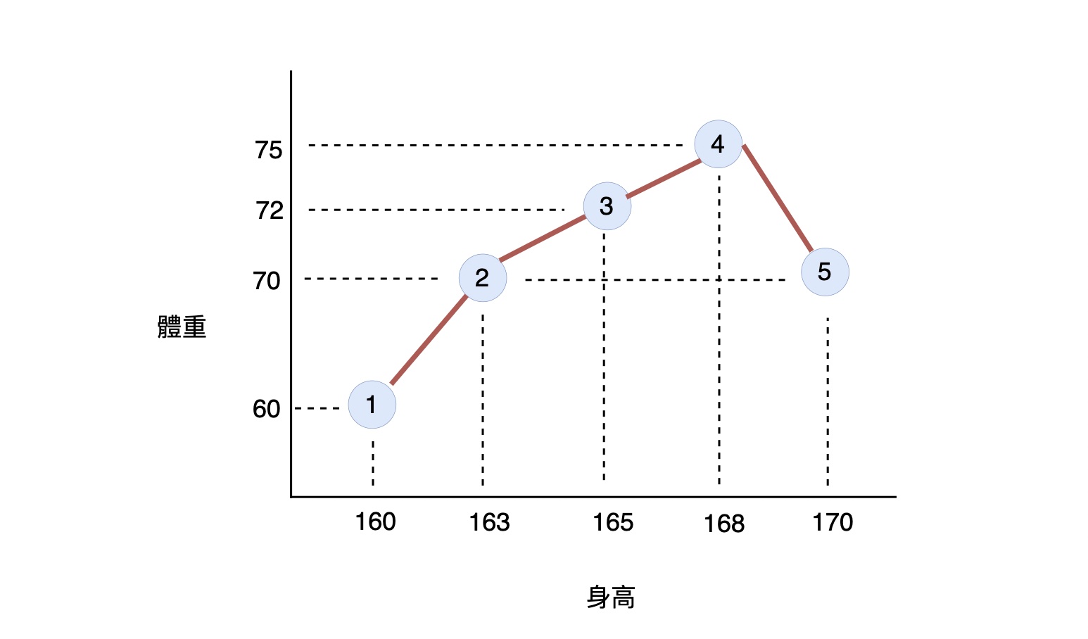
Let’s use a very small training dataset to illustrate. The dataset contains only 5 samples, each with two values: “height” and “weight”. We want to feed “height” into the model and have it output “weight” — that is, predict weight from height.
Each sample is written as (x, y), where x is height and y is weight:
- (160, 60)
- (163, 70)
- (165, 72)
- (168, 75)
- (170, 70)
Plotting these 5 samples on a 2-dimensional plane looks like this:
Suppose we train a model on this dataset — the red line in the figure below:
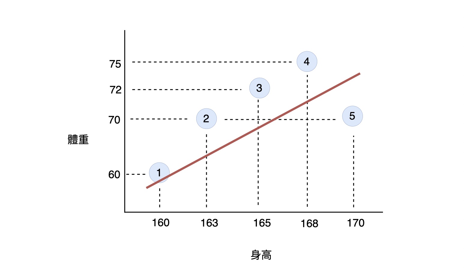
At this point we notice something: input height = 163, and the weight the model outputs is not 70. The same goes for 165, 168 and 170 — in every case the model’s answer differs from the correct one.
The error between the model’s output and the correct answer is called bias — the distance marked by the grey boxes in the figure below:
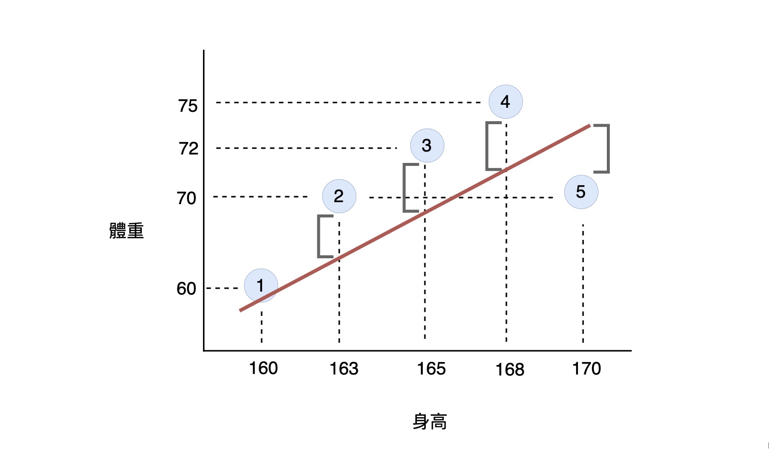
When a model’s bias is large, it means either it wasn’t trained thoroughly enough or its complexity is too low — either way, it hasn’t learned what it should have from the training dataset and simply hasn’t grasped the relationship between input and output. Give such a model a height and it may return a wildly wrong weight. We say this model is underfitting.
3 A Model’s Variance
Reading this, you’ve probably thought of a fix: “Then why not use an extremely complex model and train it until it predicts every single sample perfectly?” Follow that line of thinking and you’ll end up with a model like this:
This curve looks perfect — it hits every data point in the training dataset. The problem shows up on data it hasn’t seen: input height = 169 and the model’s output might land near 72; input height = 170 and it outputs 70; but input height = 175 and the output could drop to 60.
Heights differing by only a few centimetres, yet the model’s output swings wildly up and down. The distribution of variation in a model’s output across different inputs is called variance.
High variance means the model has swallowed everything in the training dataset whole, learning even the “noise”. Take the curve above: generally speaking, the taller someone is the heavier they are, so relative to that trend the 5th sample (170, 70) can be regarded as noise. Once the model learns that noise too, it arrives at an absurd conclusion: “the taller you are the heavier you are, but the moment you exceed 168 your weight suddenly plummets”.
Put bluntly, this kind of model has equally failed to understand the relationship between input and output — it has just rote-memorised the mapping for each individual sample. Feed it a height it has never seen and it can still give a wildly wrong answer. We call this kind of model overfitting.
4 The Bias-Variance Tradeoff
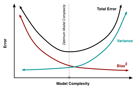
Both extremes have now appeared: too simple a model underfits, too complex a model overfits. The correspondence between these and bias/variance can be understood from the figure below:
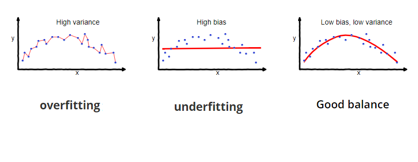
When a model is very “complex” (a large number of parameters), it has the capacity to memorise every sample in the training dataset. Variance is high and bias is low — the overfitting described above. When a model is too “simple” (a small number of parameters), it can’t learn anything at all. Bias is high and variance is low — underfitting.
Back to the sentence we opened with: a model’s total error contains both bias and variance. Since pushing one down raises the other, we have to trade off between them and find the point where total error is lowest. That is the bias-variance tradeoff.
The figure below makes this very clear:
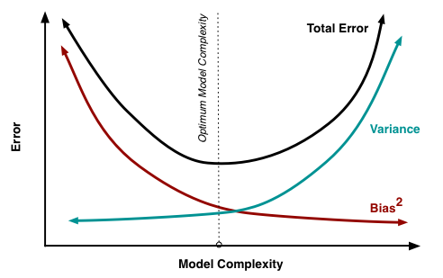
The horizontal axis is model complexity. Bias falls as complexity rises, while variance does the opposite and rises. Adding the two lines together gives a U-shaped total error. Tuning while watching only bias, or only variance, will never land you at the bottom of that U. What you’re looking for in practice is the sweet spot that minimises total error.
5 Conclusion
A model’s error is made up of bias and variance: high bias means the model hasn’t learned the relationship between input and output, which is underfitting; high variance means the model has memorised the training data along with its noise, which is overfitting. The two move in opposite directions as model complexity changes, so what you should really be chasing when tuning a model is not driving one term to its minimum, but landing total error at the bottom of the U-shaped curve.
Next time you adjust a model’s architecture or its number of training epochs, try first working out which end you’re stuck at: if the training error simply won’t come down, it’s usually a bias problem; if training performance is good but test performance is poor, then variance is the culprit.