Why Face Recognition Breaks the Old Machine Learning Playbook

1 Introduction

This is the 10th article in the “Machine Learning Fundamentals” series. In the previous posts, we walked through the five-step machine-learning workflow (Define the Problem, Prepare Dataset, Model Training, Model Evaluate, and Model Inference), and applied it to two examples: house price prediction, a Supervised Learning problem, and exploring book styles, an Unsupervised Learning problem.

Both of those used a Linear Regression Model and a K-Means Clustering Model — fairly classic machine learning models. This time we’re stepping up to a harder problem: Face Recognition. The same five steps still apply, but the piece in the middle — the model — is what has to change. A traditional model simply gets stuck on this problem, and only a neural network can actually pull it off.

2 Step 1: Define the Problem

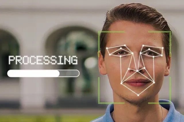
Face recognition has already worked its way into everyday life — unlocking your phone, getting through the door of your apartment building, it’s all powered by this technology behind the scenes.

Let’s set up a concrete scenario first, since every later step will come back to it. Suppose you’re someone who really cares about privacy, and you want to make sure your mischievous little brother can’t just wander into your room while you’re at work during the day. Cutting yourself a spare key feels like too much hassle, because you know you’ll lose it. So instead, you decide to build a face recognition system: the electronic door lock only opens when it recognizes “this is you.”

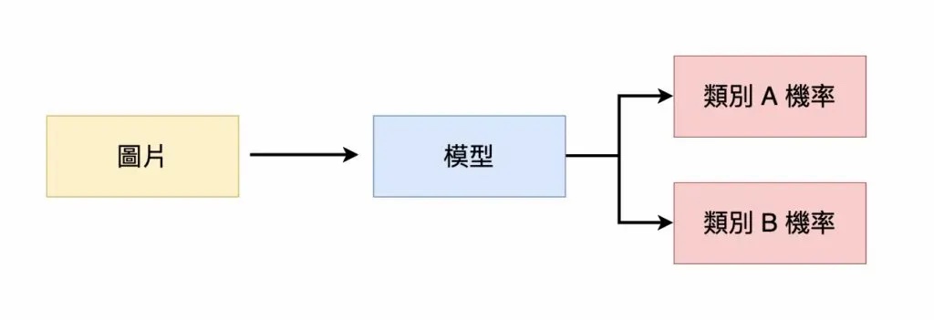
To build this system, the core task is training a model that can tell “your face” apart from everyone else’s. The input is “an image,” and the output is the “class” that image belongs to. We define two classes up front:

• Class A: the image contains your face
• Class B: the image does not contain your face

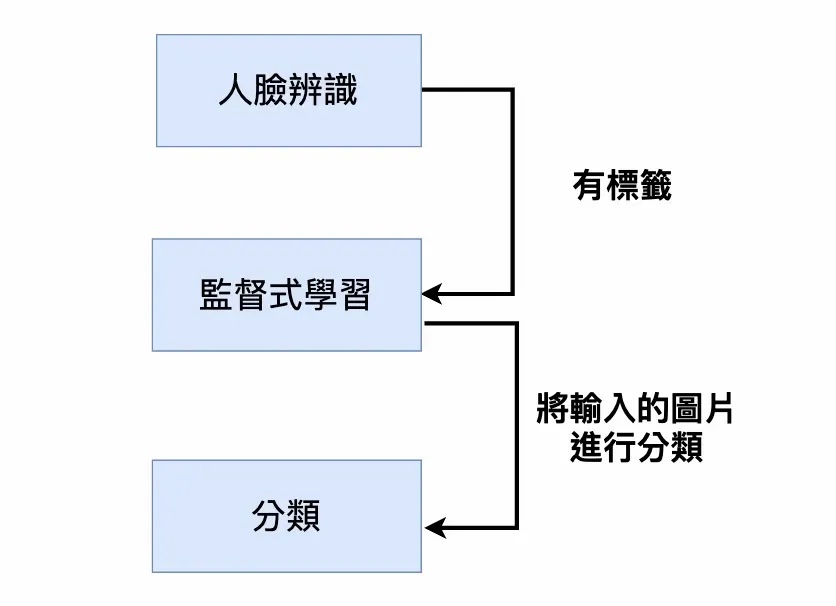
To train this model, we need a large number of images, each labeled as either Class A or Class B. Because these images are labeled with their correct class in advance — essentially a correct answer sitting right next to the model as it learns — this problem is Supervised Learning. And because the model’s output is a “class” rather than a continuous value, the task type is Classification.

Defining the problem might sound like stating the obvious, but it decides how the next three steps get done: knowing it’s supervised learning tells you the data has to be labeled; knowing it’s a classification task tells you evaluation should look at accuracy, not error values.

3 Step 2: Prepare Dataset

Preparing the dataset can be roughly broken into four stages.

• Data Collection If you want to train a model “from scratch,” you need a large number of already-labeled images. If you don’t have enough data, the model is prone to “Overfitting” during training — in plain terms, the model ends up memorizing the training data, doing great on questions it’s already seen but starting to guess wildly the moment it sees a new, unseen photo. Data Augmentation techniques can help here: rotating, flipping, cropping, and adjusting the brightness of existing images to generate more varied training samples.
• Data Exploration and Data Cleaning The quality of the dataset directly caps how good the model can get, so this step is about improving image quality and making sure the labels are correct wherever possible — for example, weeding out blurry photos and checking that no label was misapplied. You can also write a script to standardize every image’s size and format, which makes training easier later on.
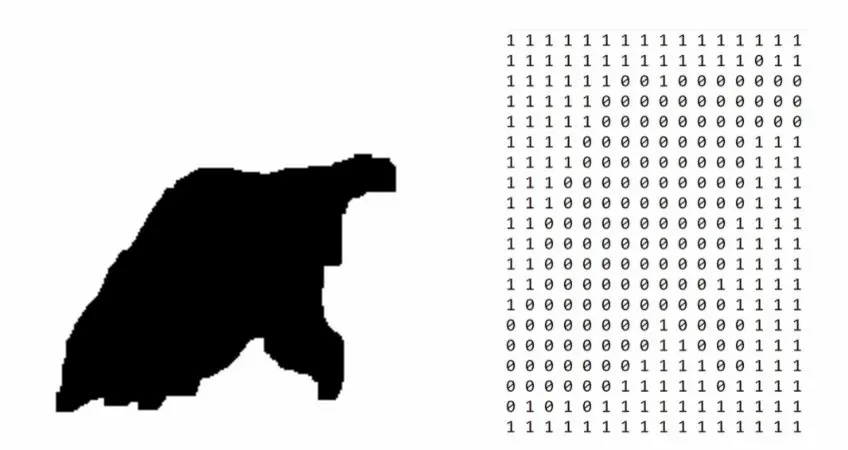
• Data Vectorization A model consumes “numbers,” not “images,” so images have to be converted into matrices first. In the example below, the left side is a black-and-white image, and the right side is the matrix representing it, where 0 means the pixel is “black” and 1 means it’s “white.” A color image is made up of three RGB channels, so it gets represented by three matrices instead.

• Split Data After the model is trained, we need “data the model has never seen” to evaluate how good it actually is, so the full dataset gets split into a Training Dataset and a Testing Dataset up front, with 80% : 20% being a common ratio. Train on the Training Dataset, evaluate on the Testing Dataset. Evaluating with data the model was already trained on would be like letting a student grade the exact exam paper they’d just finished checking against the answer key — a high score there tells you nothing.

4 Step 3: Model Training

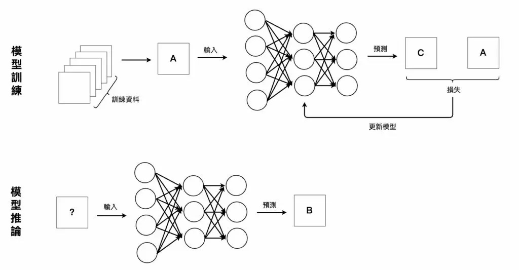
The previous two articles used classic machine learning models (a Linear Regression Model and a K-Means Clustering Model), but for face recognition, we switch to a Neural Network model instead.

The reason is straightforward: a traditional model needs a human to hand it “meaningful features” ahead of time, but human faces are simply too hard to describe with hand-written rules — eye spacing, skin tone, facial contours, on top of every possible angle and lighting change. You could spend a lifetime writing rules and still not cover it. A neural network’s strength is learning those features on its own straight from the raw pixels, which is exactly why it can handle a broader, harder class of problems than a traditional model. The inner workings of neural networks themselves are outside the scope of this article — a dedicated post will cover that later.

Neural networks come in many flavors, each good at a different kind of task. Back in the problem-definition step, we already framed face recognition as “Image Classification,” and for image inputs specifically, the Convolutional Neural Network (CNN) is the go-to choice. A CNN excels at extracting the important features in an image — edges, contours, and other local patterns — and combining them layer by layer into progressively more complete concepts, which is what drives up an image classification model’s prediction accuracy.

5 Step 4: Model Evaluate

Once training is done, we measure quality using the Testing Dataset together with Statistical Metrics. The most intuitive one is Accuracy — simply the fraction of predictions the model got right.

But looking at Accuracy alone can be deceiving. Back to our door-lock scenario: if the camera’s view is empty (Class B) most of the time, a model that learns nothing at all and just always answers “not you” can still rack up a very high Accuracy score — yet it’s completely useless, because you’d never be able to get into your own room. This exact failure mode is why metrics like the Confusion Matrix, Precision, Recall, and the ROC Curve exist — we’ll leave those for a future article.

6 Step 5: Model Inference

Once the model clears evaluation, it can officially go live as your “room guard.” Every time the camera takes a picture, it gets fed into the model, the model predicts a class, and the system takes the corresponding action based on the result.

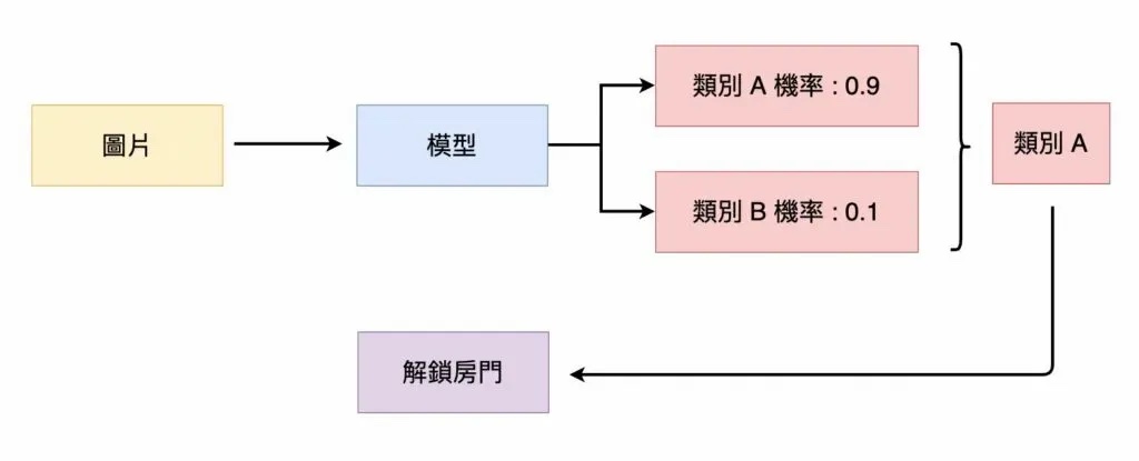
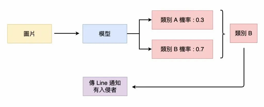
If Class A comes back with the higher probability, the door unlocks; if Class B comes back higher, the alarm sounds. This is where the five steps finally close the loop: the problem we defined at the start ends up as a system that actually makes decisions.

7 Conclusion

This article walked through the five-step machine-learning workflow once again, this time solving “face recognition.” Recognizing faces has always been a genuinely hard task for computers — it took the arrival of the neural network to push accuracy high enough for face recognition to actually land in everyday scenarios like unlocking phones and building access control.

Looking back across the whole series, the five steps themselves never change — only the model in the middle does. The next article will head into neural network territory and take a closer look at how they actually work.