Deep Learning Fundamentals: An Introduction to Gradient Descent

1 Introduction

In “The Principles of Deep Learning: How a Neural Network Classifies Images”, we used the classification of handwritten digit images as an example to get a feel for how a neural network understands an image. We then learned that a neural network relies on the following 3 elements to adjust its internal parameters (weights and biases) so that its output gets closer and closer to the correct answer:

• Training dataset
• Cost function
• Optimizer

The first two were covered in Deep Learning Fundamentals: The MNIST Dataset and the Cost Function. This article covers the third element — the optimizer — and specifically the most basic and most important one of all: gradient descent. By the end of this article you will know what gradient descent actually does, what the mathematics behind it looks like, and what role the learning rate plays in it.

2 What Are We Actually Training When We Train a Neural Network?

Before getting into the algorithm, let’s be clear about what “training” means. Training a neural network is, put plainly, adjusting the parameters inside the network (weights and biases) to a good set of values, so that the network’s output is as close to the correct answer as possible.

So how do we measure “good” versus “bad”? That’s what the cost function is for.

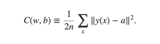
The cost function condenses “how well the current set of parameters is doing” into a single number: the smaller the value, the closer the network’s output is to the correct answer. So the process of training a neural network is really about adjusting w (weight) and b (bias) to minimise the value of C (the cost function).

In one sentence: training a neural network ⇒ adjusting the parameters (w and b) so that the cost function gets smaller.

Which raises the question: how exactly should we adjust w and b to make the cost function smaller and smaller? That’s what the gradient descent algorithm is for.

3 Understanding Gradient Descent Through a Valley and a Ball

To make the concept clear, let’s simplify the problem first. Forget for a moment about neural networks, cost functions, weights and biases.

All we have now is a function $C(v)$, where $v = v_1, v_2, \dots$, meaning C can take any number of parameters. The goal is simple: use gradient descent to adjust each v so that the value of $C(v)$ gets smaller and smaller.

To make it easy to visualise, let’s assume C takes only two parameters, $v_1$ and $v_2$ — that is, $C(v_1, v_2)$. Different inputs $v_1$ and $v_2$ give different values, and if we plot every $(v_1, v_2) \Rightarrow C(v_1, v_2)$ case, those points form a surface in 3-dimensional space:

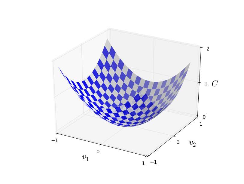
Looking at the figure above, you can probably spot the minimum at a glance. But in practice a neural network easily has tens of millions of parameters, so eyeballing it is out of the question. This is exactly where gradient descent comes in.

Before the mathematics, let’s take a more real-world perspective: think of the function $C(v)$ as a “valley”, and think of ourselves as a “ball” somewhere on it. How does a ball move? It rolls down the slope, of course, and doesn’t stop until it reaches the bottom.

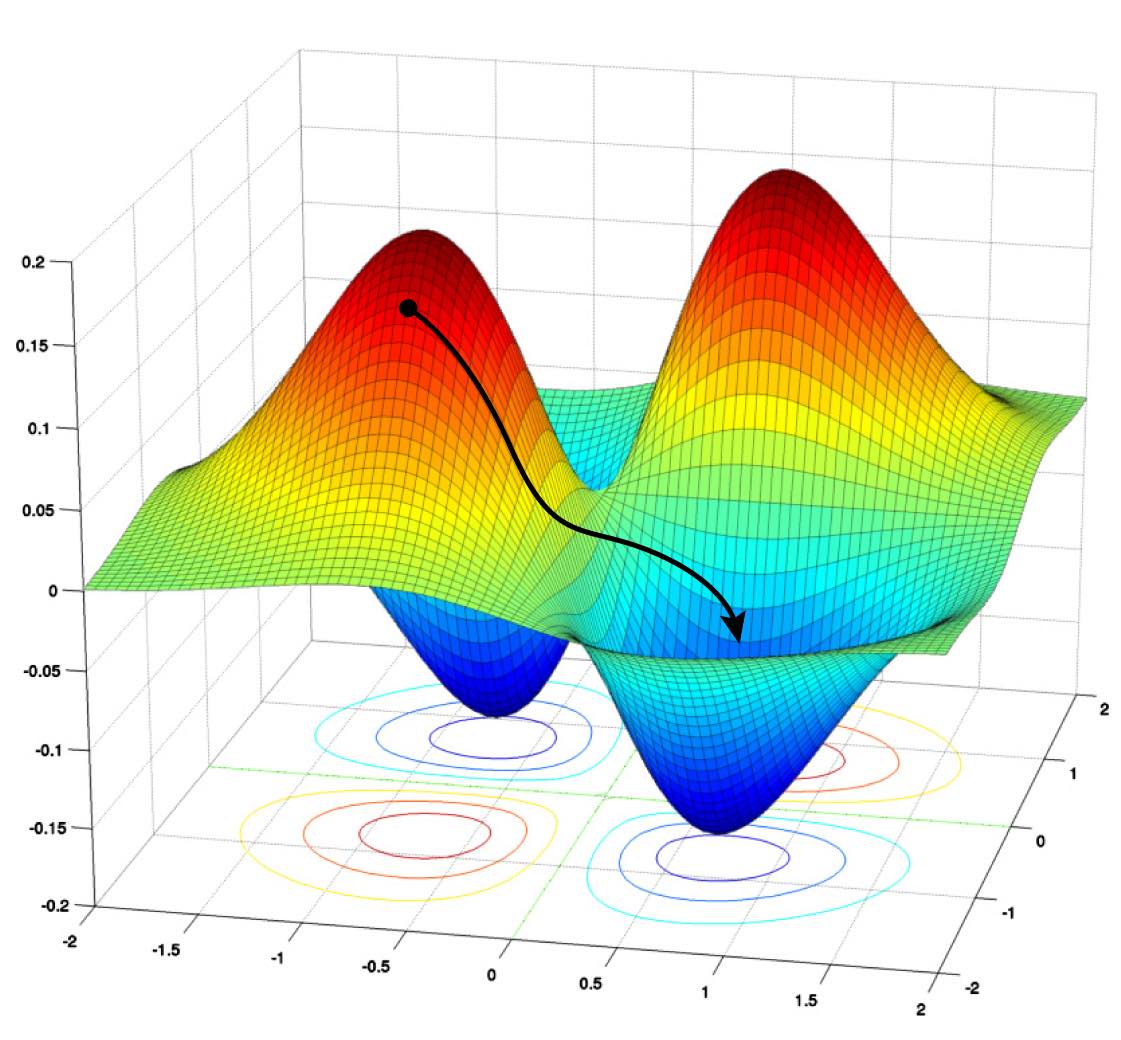
Here’s the catch: we are a ball resting on the hillside, the valley’s terrain is complicated (as shown above), and we cannot see where the bottom is — we only know how the terrain changes near our “current position”.

Given that, the only way to reach the bottom is a brute-force approach: feel out which of the surrounding directions is “downhill”, take a step that way; once at the new position, feel out the downhill direction again and take another step… and repeat, until every direction around us is flat and no downhill direction can be found. At that point we’re at the bottom.

4 The Mathematics of Gradient Descent

With the “valley and ball” analogy in place, let’s fill in the mathematics. This won’t go to maths-department depth — a little understanding of partial derivatives is enough.

Back to $C(v) = C(v_1, v_2)$. Where the ball starts depends on the initial values of $v_1$ and $v_2$. Because we’re treating ourselves as the ball, we can’t see the whole valley and therefore can’t see where the lowest point of $C(v_1, v_2)$ is — we only see the state of our current position.

Suppose we’ve decided to move in some direction (represented by the vector $\Delta v$). We can break that step into first moving $\Delta v_1$ along the $v_1$ direction, then $\Delta v_2$ along the $v_2$ direction — that is, $\Delta v \equiv ( \Delta v_1, \Delta v_2 )^T$ (where T means transpose).

After taking one step along $\Delta v$, the change in $C(v_1, v_2)$ is called $\Delta C$, and can be written as the following equation:

The concept of partial derivatives was introduced in An Improved Perceptron: Understanding the Sigmoid Neuron. Here you can simply think of it as the “rate of change” of a multivariable function with respect to one independent variable. For example, when $v_1$ increases by 5 ($\Delta v_1 = 5$), the effect on C is not necessarily an increase of 5 ($\Delta C$ doesn’t necessarily equal 5) — it must be multiplied by C’s rate of change with respect to $v_1$ (how much C changes when $v_1$ changes by 1).

Next, we extract the partial-derivative part of the $\Delta C$ equation and give it a new symbol, $\nabla C$, called the “gradient of C”:

Don’t be alarmed the first time you see the $\nabla$ symbol. $\nabla$ is generally used to denote a gradient vector, and a gradient vector isn’t anything remarkable — it’s just a vector in which every element is a partial derivative (the derivative of the function with respect to one particular parameter).

With $\Delta v$ and $\nabla C$ in hand, the original $\Delta C$ equation can be rewritten as:

This equation makes it clearer: $\Delta C$ (the change in the function) is determined by the product of $\Delta v$ (how much each parameter moves) and $\nabla C$ (the effect on C of moving each parameter by one unit).

Don’t forget our goal. We’re a ball, and we want the value of $C(v_1, v_2)$ to decrease after moving by $\Delta v$ — that is, $\Delta C \leq 0$. So how do we pick $\Delta v$? Simply set:

Substituting gives $\Delta C \approx -\eta \nabla C \cdot \nabla C = -\eta \|\nabla C\|^2$. Because $\|\nabla C\|^2$ is always greater than or equal to 0, $\Delta C$ is guaranteed to be less than or equal to 0 — this step is guaranteed not to go uphill.

At this point we know how to take each step. When the ball is currently at v and moves to a new position v':

Following this rule, we recompute $\nabla C$ (the gradient vector) for every step we take, and $C(v_1, v_2)$ gets a little smaller with every move. Step by step we keep going until we reach the bottom of the valley — the minimum of $C(v_1, v_2)$. This whole process is what’s called gradient descent.

5 What Is η (the Learning Rate)?

There’s one symbol in the equation above we haven’t explained: $\eta$. In machine learning, $\eta$ stands for the learning rate.

To understand what the learning rate means, let’s look again at what $\nabla C$ (the gradient vector mentioned earlier) does. $\nabla C$ records the function’s partial derivatives with respect to each parameter. In the case where C has only one parameter v, this is really just computing the slope of the tangent line, and the slope tells us which direction each parameter should move in. If C’s partial derivative with respect to v is “negative”, it means C “decreases” as v increases; if the partial derivative is “positive”, it means C “increases” as v increases.

So the division of labour is clear: $\nabla C$ determines each parameter’s “direction of movement”, and $\eta$ (the learning rate) determines the “size of the movement”.

In deep learning, $\eta$ is a kind of hyperparameter, meaning we have to set and tune it ourselves — it cannot be tuned automatically by the neural network’s learning process.

Choosing the value of the learning rate is an art in itself, and both extremes cause problems:

• Learning rate too large: v changes too much at once, and in some cases this actually makes $\Delta C$ greater than 0, sending the value of C higher and higher. In the valley analogy, the step is so big that you jump straight from this hillside over to the opposite one.
• Learning rate too small: v changes only a tiny amount each time. The direction is right, but it takes an enormous number of steps and a great deal of time to reach the minimum.

6 Gradient Descent: From Two Variables to Many

Everything so far has been explained using the two-variable $C(v_1, v_2)$. A real neural network is of course not that simple, but here’s the good news: if you understood everything above, you already understand how gradient descent applies to deep learning.

The only difference is that there are more variables: the two-variable cost function $C(v_1, v_2)$ becomes a many-variable $C(v_1, v_2, v_3, v_4, \dots)$. When we move by $\Delta v$, it still produces a change $\Delta C$, and the relationship between the two is exactly the same as before:

It’s just that $\Delta v$ now contains more elements: $\Delta v \equiv ( \Delta v_1, \Delta v_2, \Delta v_3, \Delta v_4, \dots )^T$, and $\nabla C$ likewise goes from two elements to many:

In the two-variable example, we chose $\Delta v = -\eta \nabla C$ for every step. In the many-variable case we choose exactly the same thing, and update v with exactly the same rule, driving the cost function’s value lower and lower. The entire logic is unchanged — the vector just got longer.

7 Conclusion

This article introduced the concept of gradient descent. Stripped down, gradient descent is about computing a function’s gradient vector to learn the direction in which to update the parameters, so that the function’s value gets smaller and smaller.

We also covered the learning rate: a hyperparameter that must be set in advance. Computing the gradient gives us the parameters’ “update direction”, while the learning rate lets us decide the parameters’ “update size” — neither works without the other.

Now that you understand gradient descent, the next article covers its practical variant: Stochastic Gradient Descent.

7.1 References

• Gradient descent – Wikipedia
• Neural networks and deep learning
• Gradient Descent Algorithm — a deep dive | by Robert Kwiatkowski | Towards Data Science
• Gradient Descent — ML Glossary documentation (ml-cheatsheet.readthedocs.io)
• An overview of gradient descent optimization algorithms (ruder.io)