Deep Learning Fundamentals: The MNIST Dataset and the Cost Function

1 Introduction

In the previous article, “Classifying Handwritten Digit Images with a Neural Network”, we designed a neural network for the handwritten-digit classification problem and got a feel, from the network’s point of view, for how it understands an image: the input layer stands for each pixel in the image, the hidden layer learns to capture the image’s important features, and the output layer then classifies the image based on the features that were captured.

Designing the architecture, though, is only the first step. The parameters inside the network (the weights and biases) all start out random, and getting the output to become more and more accurate depends on the following 3 elements:

• Training dataset
• Cost function
• Optimizer

This article covers the first two: the training dataset and the cost function. With data, the neural network has something to learn from; with a cost function, we have a way to judge “how good is the current set of parameters, really?” As for how to adjust the parameters based on that judgement — that’s the optimizer’s job, and it’s left for the next article.

2 An Introduction to the MNIST Dataset

To train a neural network, what you cannot do without is a large pile of training data. For the handwritten-digit classification problem, the most famous dataset is the MNIST dataset, which contains tens of thousands of handwritten digit images along with the correct label for every image.

MNIST stands for Modified National Institute of Standards and Technology database. It is a modified version of two datasets created by NIST.

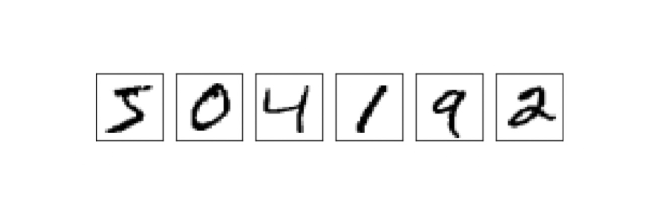
The MNIST dataset consists of 2 parts: the training data and the test data. The training data contains 60,000 handwritten digit images, written by 250 people — 50% of them high school students and the other 50% employees of the Census Bureau — which ensures the handwritten digit images in the training data cover as many different handwriting styles and characteristics as possible.

The test data contains 10,000 handwritten digit images. These likewise come from American high school students and the Census Bureau, but they are the handwriting of a different set of 250 people. That “different people” part is crucial: if the handwriting in the test data came from the same group as the training data, the model scoring well might just be because it has seen similar handwriting before. Switching to people it has never seen is the only way to really judge whether the neural network can genuinely classify the images correctly.

In the MNIST dataset, every image is a “grayscale” image made up of 28 × 28 pixels, and every image has a corresponding label stating which digit it represents.

In the previous article’s neural network design, we mentioned that the input layer would contain 784 neurons — and that number comes precisely from 28 × 28. Because we are designing the most elementary, most basic neural network, in practice we flatten each image from a 28 × 28 2-dimensional matrix into a 1-dimensional vector of 784 elements, and use x to denote the image fed into the neural network (so x is a 784-dimensional vector).

We use y(x) to denote the actual digit that the image corresponds to. What’s unusual is that y(x) is not a single number, but a 10-dimensional vector:

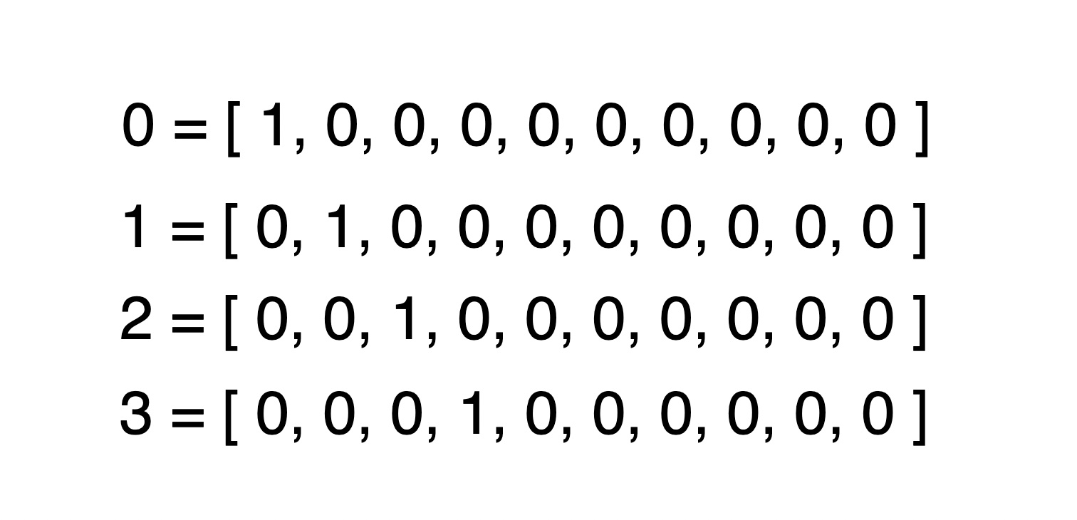
If the digit in the image is 0, then the 1st number in the 10-dimensional vector is 1 and the rest are 0; if the digit is 1, then the 2nd position is 1 and the rest are 0, and so on. A y(x) of this shape fits our design of the neural network’s output layer rather well. The output layer already has 10 neurons, each representing the degree to which “this image is a particular digit”, so using a 10-dimensional vector as the answer lines up one-to-one.

Representing the digits 0 through 9 (these 10 categories) with vectors like the ones above is a common way of encoding categorical data in machine learning, known as one-hot encoding.

3 The Neural Network’s Goal: Minimising the Cost Function

With the MNIST training dataset in hand, we want the neural network to learn the correct parameters (weights and biases) from that training data. Put plainly: we feed in an image x (a 784-dimensional vector), the neural network outputs a y (a 10-dimensional vector), and we want that y to be as close as possible to y(x) (the actual digit x corresponds to, also a 10-dimensional vector).

The way a neural network “adjusts” its parameters is through an optimizer. That optimization algorithm is also the most interesting and most valuable part of deep learning, and we’ll go into it in depth in later articles.

There’s a prerequisite before any adjusting can happen, though: if we want the optimizer to adjust the neural network’s parameters properly, we need some way of judging how good the network’s current parameters are. The tool used for that is called the cost function.

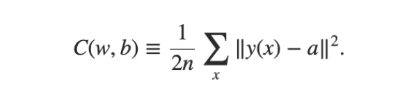
As the figure above shows, the cost function C is a function that takes two values: w and b. w stands for all the weights in the neural network, and b stands for all the biases. Given w and b, C (the cost function) computes a number representing how good or bad that set of w and b is. In the equation above, x denotes one piece of training data (one image); y(x) denotes the actual digit that image corresponds to; a is the output after feeding x into the neural network; and ‖v‖ denotes the length of the vector (y(x)-a).

Here a depends on x (the image currently being fed in) and on w, b (the parameters in the neural network). A good neural network is made up of good parameters (w and b) such that, for most inputs x, it produces an a close to y(x), making the value of ‖ y(x) – a ‖ smaller.

So we can use a cost function to measure how good the parameters are: the lower the cost function’s output, the better the current set of parameters; conversely, the higher the cost function’s output, the worse the current set of parameters.

With a cost function in place, the optimizer’s goal becomes perfectly clear: minimise the cost function. The optimizer has to try to find a set of w and b that “minimises” the cost function’s output. And the optimizer we use is called gradient descent.

4 Conclusion

In this article we came to understand the roles that the training dataset and the cost function play in deep learning: MNIST provides 60,000 training images and 10,000 test images, each image is flattened into a 784-dimensional vector x, and the answer is expressed as a 10-dimensional y(x) using one-hot encoding; the cost function is responsible for condensing “how good is this set of w and b?” into a single comparable number.

In other words, what we call a neural network’s “learning” is really about using an optimizer to find a set of weights and biases that minimises the cost function’s output.

In the next article, we’ll learn the concept of the optimizer in deep learning, starting with the most basic optimizer of all — gradient descent.

4.1 References

• Neural networks and deep learning
• MNIST database – Wikipedia
• One-hot – Wikipedia