Machine Learning Problem-Solving in 5 Steps: Model Training


1 Introduction
This is the fifth post in the “Machine Learning Fundamentals” series. In the previous post we talked about preparing a dataset — how to put one together, and why it sets a hard ceiling on how good your model can ever get. Once the dataset is ready, the next step is the subject of this post: model training.

This post first pins down what “training a model” actually means, then walks through a few terms you’ll run into once you start writing code: hyperparameters, the Python libraries people actually use, and the common categories of models.
2 From dataset to model training
Once a dataset is ready, we don’t usually feed the whole thing into training as one block — we split it into two parts first: a training dataset and a test dataset.
The training dataset, as the name suggests, is what the model actually learns from. Once training is done, we want to know how good the model really is. If we quiz it using data it already saw during training, the score doesn’t mean much — it’s like grading a student on an exam they already saw the answers to. That’s why we deliberately hold back a portion of data the model has never seen: the test dataset, used to check the model’s real-world performance.
3 What model training actually means
In our earlier post on “models, training, and inference in machine learning,” we explained that a “model,” in machine learning, is really just a “function.” A function takes an input, runs some computation, and returns an output — and inside that function are a bunch of “parameters” that determine exactly what the output looks like.
With that in mind, model training can be summed up in one sentence:
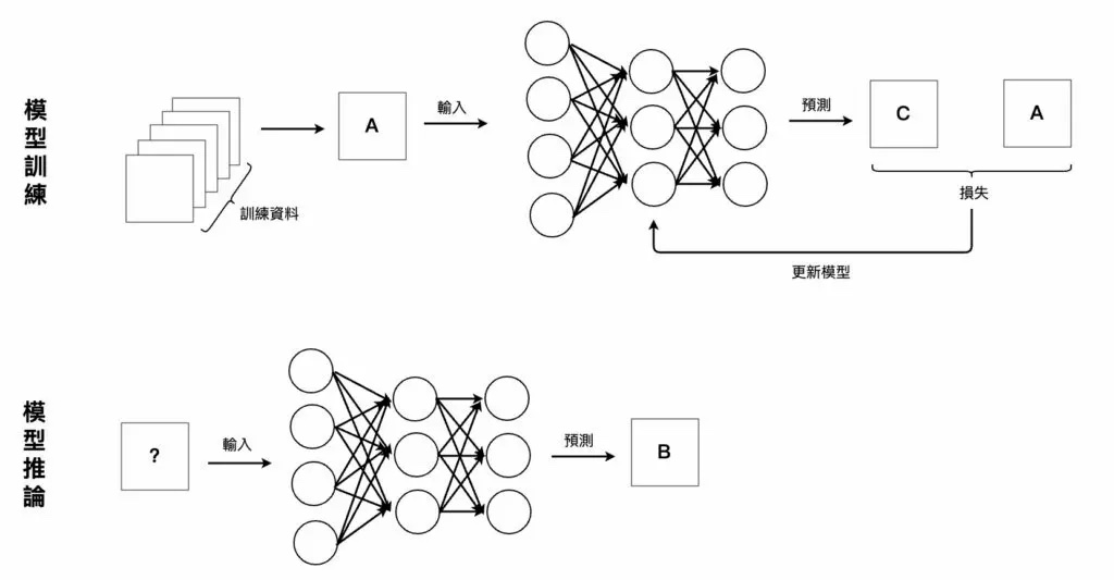
Repeatedly adjust the model’s parameter values, using some method, so that the model’s output gets more and more accurate — in other words, minimize the loss function.
Two key terms show up in that sentence: parameters and the loss function. Let’s take them apart one at a time.
Parameter: a model is a function, and inside that function are a number of parameters that combine with the input to produce the output. For example, take the function F1(x) = 3x + 5 — the 3 and the 5 are this function’s parameters. Feed in 6, and the function outputs F1(6) = 23. A function can of course be more complex, with more parameters — for example F2(x) = 3x² + 2x − 10, where 3, 2, and −10 are all parameters. Feed in 1, and you get F2(1) = −5.
Loss function: the loss function is the key piece of model training — its job is to measure “how bad is this model right now.” Take F2(x) above: each of its three parameters could be swapped for millions of different numbers, and we need to pick out the best combination. That’s exactly what the loss function is for. Since it’s also a function, it has its own input and output:
Loss Function(model’s parameters) = how bad the model is
Feed the model’s current parameters into the loss function, and it tells you how bad that particular combination is. The larger the output, the worse the model. So the training goal is intuitive: push that number down.
A house-price example makes this more concrete: the model predicts a house is worth 10 million, but it actually sells for 12 million — that 2-million gap is exactly what the loss function is meant to quantify. The smaller that gap is across the whole training set, the better the chosen parameters are.
4 The training loop
Putting all of that together, training a model really just means repeating three steps over and over:
- Feed the training dataset into the model.
- Use the loss function to measure how good (or bad) the current model is.
- Update the model’s parameters so the loss function’s value goes down (i.e., improve the model).
Run one pass, compute the loss once, adjust the parameters once, then run the next pass. When does it stop? That’s a decision we make ourselves — it might be after a fixed number of iterations (say, 10,000), or once the loss drops below some threshold.
5 Hyperparameters during training
Now that the training loop makes sense, let’s look at a term you’ll actually run into when writing code: the hyperparameter.
When building and training a model, some values have to be set by hand — the model itself can’t learn or adjust them during training. These are hyperparameters. The simplest example is the “number of training iterations” mentioned above: how many rounds to run is a decision we make ourselves, whether that’s a fixed number based on experience, or a stopping condition that halts training once it’s met.
So there are two kinds of “parameters” that are easy to mix up — remember this distinction and you’re set: a model’s parameters are the values automatically adjusted during training; hyperparameters are the values we have to set before training starts, and they don’t change on their own during training.
6 Common Python libraries
When it’s time to actually build or train a model, there’s no need to code everything from scratch — plenty of ready-made packages and frameworks exist.
For traditional (non-deep-learning) machine learning models, the most commonly used library is:
For deep learning models, the common libraries are:
- TensorFlow
- PyTorch
- MXNet (note: MXNet has since been retired to the Apache Attic — new projects should go with PyTorch or TensorFlow instead)
We won’t go deeper into any of these here — there’s already excellent documentation online covering how to use them and the design ideas behind them.
7 Common model types
In our post on defining the problem, we talked about identifying which kind of machine learning task a “problem” actually is, so you can build the right kind of model for it. In practice there are an enormous number of model types out there, and “picking a model” is itself a trial-and-error process. Here we’ll group them into three broad categories.
- Linear model
Most of the models introduced in this beginner series fall into this category. These models tend to be relatively simple and can be expressed directly as a single mathematical function — for example F(x) = 2x³ + 3x² − 10x + 5, where different values of x produce different outputs. In the “defining the problem” post, we used a house-price prediction example to illustrate exactly this: this kind of model is suited to “linear regression” problems, which is why it’s also called a linear regression model.
What about classification problems — can a linear model still handle those? Absolutely. Take “binary classification” as an example — sorting input data into class A or class B. We can take the output of a linear regression model and pass it through another function so the output always lands somewhere between 0 and 1, then treat that 0–1 number as the probability of belonging to one of the two classes.
A linear regression model with this extra transformation added on top is exactly what’s called a logistic regression model.
- Tree-based model
Tree-based models also show up frequently in this series. The idea is to use a “tree”-like structure that splits the input data one level at a time, eventually arriving at a result.
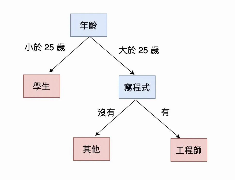
For example, say we have a person’s basic profile — height, blood type, interests, expertise, age, and so on — and we want to predict their occupation. The reasoning might look like this:
- Is the person older than 25? If not, they’re “a student.” If so, they’re “not a student.”
- Do they write code? If yes, they’re “an engineer.” If not, they’re “something else.”
Drawn out as a tree, that chain of reasoning looks like this:
- Deep learning model
Deep learning models have been an especially hot topic in recent years. They mimic the structure of the human “brain,” building a model out of layer after layer of “neurons.” Deep learning models come in an enormous variety too, and different task types call for different architectures. Here are a few of the most common:
Feed Forward Neural Network (FFNN): the earliest and simplest kind of neural network, stacking neurons layer by layer, with information passed downward between layers through weights.
Convolutional Neural Network (CNN): good at extracting useful information from images, and widely used in image-processing tasks.
Recurrent Neural Network (RNN): good at extracting useful information from sequential, time-based input data, and widely used in natural language processing tasks.
8 Conclusion
This post covered what “model training” actually means — breaking apart the two core concepts of parameters and the loss function — and rounded up a few things you’ll run into in practice: hyperparameters, commonly used libraries, and the main categories of models.
Honestly, the second half of this post is already fairly advanced material, so it’s completely normal if it doesn’t all click on a first read — don’t get discouraged. These terms will keep coming up in later posts, and they’ll feel a lot more familiar the more you see them.
In the next post, we’ll move on to what happens after training is complete: model evaluation.