An Improved Perceptron: Understanding the Sigmoid Neuron

1 Introduction

In the previous article, “Understanding the Perceptron”, we met the oldest artificial neuron of all — the perceptron — and looked at its mathematical formulation as well as its relationship to the NAND gate. But the perceptron is not the neuron that modern neural networks actually use.

This article introduces a neuron that is much “closer” to modern neural networks: the sigmoid neuron. We’ll start from the question of how a neural network actually learns, look at where the perceptron gets stuck, then explain what modification the sigmoid neuron makes, why that modification happens to solve the problem, and finally how its output should be interpreted. You don’t need to have read the previous article — every concept you need is covered here.

2 How a Neural Network Learns

The reason a perceptron is more than just an incarnation of a NAND gate is the existence of a learning algorithm, which lets the neuron tune its own parameters (weights and biases) to the right values. Before actually designing a learning algorithm, let’s build a more intuitive understanding of how a neural network learns to produce the correct output.

Take a very concrete task: a neural network whose input is a photo of a handwritten digit, and whose output is the digit that photo represents.

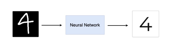
A neural network’s parameters start out randomly generated, so its initial outputs are usually terrible. Feed it a handwritten 4 and it might call it a 6. To produce correct results, it has to keep adjusting its parameters.

And here is the property we’d really like to have: every “slight” adjustment to a parameter produces only a “slight” change in the output.

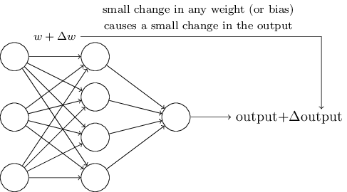
As shown above, we add a very small $\Delta w$ to some parameter $w$ in the neural network, and the output changes by a correspondingly small $\Delta \text{output}$. If that really holds, learning becomes much easier: suppose feeding in a photo of a handwritten 9 gives us an output of 8 — we only need to work out which direction each parameter should move in (up or down), nudge it a little, and we can expect the output to move a little in the right direction too. Keep doing that until the output becomes 9.

In other words, the “small parameter change → small output change” property is a prerequisite for the whole learning process to converge stably.

3 The Problem the Perceptron Brings

The problem is that the perceptron does not have this property. Let’s go back to its basic structure:

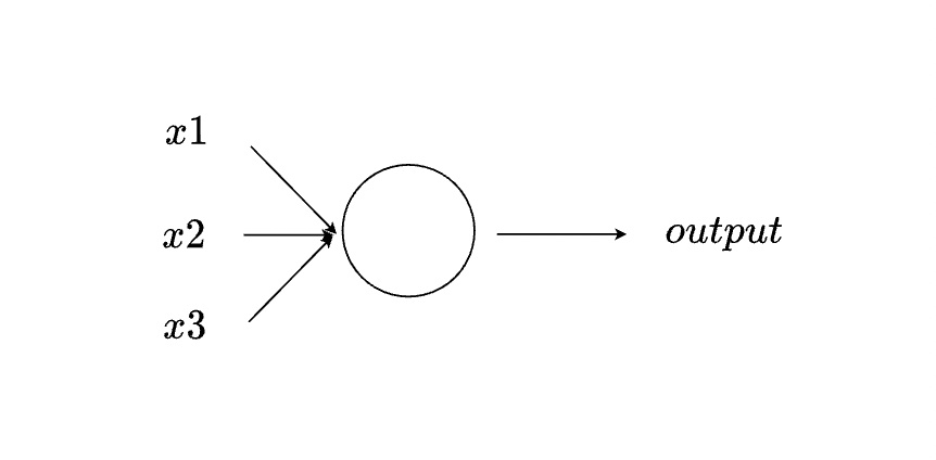
A perceptron takes several binary values as input and produces a binary value as output. A “binary value” is either 0 or 1 — there is no grey area in between.

That’s exactly where the trouble comes from. In a neural network made up of many perceptrons, even a “small” adjustment to one perceptron’s weight can flip that perceptron’s output outright, from 0 to 1. And that perceptron’s output is in turn an input to other perceptrons further along, so the flip propagates and the whole network’s output becomes unpredictable.

To be concrete: we feed in a photo of a handwritten 9 and get an 8. We repeatedly nudge the parameters until it finally outputs 9 correctly. But along the way, many perceptrons in the network have had their outputs flipped entirely (0 to 1, 1 to 0), so other photos that used to be classified correctly may now come out wrong. Fix one, break a dozen — learning simply cannot accumulate.

4 Enter the Sigmoid Neuron

To make a neuron’s output capable of changing by small amounts, a new artificial neuron was proposed: the sigmoid neuron. It isn’t a from-scratch redesign — it’s a small modification to the perceptron.

A sigmoid neuron looks exactly like a perceptron (compare the perceptron diagram above): it takes several inputs x1, x2, x3 and produces one output. What is genuinely different is the type of those values.

In a perceptron, the inputs can only be discrete binary values, 0 or 1. In a sigmoid neuron, the inputs are any number continuously distributed between 0 and 1 — 0.2556 or 0.6398, for instance. Just as before, each input is multiplied by its own weight and summed, and a bias is added, producing a final value.

As shown above, a perceptron compares that final value against a threshold, and the output is 0 or 1. A sigmoid neuron is different: like its inputs, its output is any number continuously distributed between 0 and 1. More precisely, a sigmoid neuron passes the final value $(w \cdot x + b)$ through a sigmoid function before emitting it, so its output is $\sigma(w \cdot x + b)$.

That “$\sigma$” is called the sigmoid function, and its full formula is:

To recap the sigmoid neuron’s computation: first multiply every input x by its corresponding weight and sum them, then add the bias, giving $z = w \cdot x_1 + w \cdot x_2 + w \cdot x_3 + \cdots + bias$; then feed $z$ into the sigmoid function and output $\sigma(z)$.

5 Where the Sigmoid Neuron and the Perceptron Are Alike

When you first meet the sigmoid neuron, it’s easy to assume that the extra sigmoid function makes its output very different from a perceptron’s. In fact the opposite is true — the two behave very similarly most of the time.

Suppose $z = w \cdot x + b$ is a large positive number. Then $e^{-z}$ approaches 0, and $\sigma(z)$ works out to approach 1. In other words, when $z$ is large the sigmoid neuron outputs 1, exactly like a perceptron.

Conversely, when $z = w \cdot x + b$ is a large negative number, $e^{-z}$ approaches infinity and $\sigma(z)$ approaches 0 — again, exactly like a perceptron.

The only place they genuinely differ is when $z$ is neither large nor small, but sits somewhere in the middle. And that “grey zone” is precisely where the sigmoid neuron’s value lies: it takes what was a cliff between 0 and 1 and paves it into a gentle slope.

6 The Sigmoid Function’s Most Important Property: Smoothness

We won’t go deep into deriving the details of the sigmoid formula. The focus is on its most critical property: smoothness.

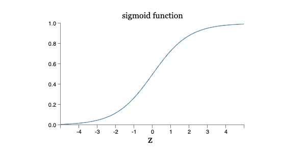
The figure above is what the sigmoid function looks like plotted on a two-dimensional plane. Put it side by side with the step function and you’ll see that the sigmoid function is simply a “smoothed” version of the step function:

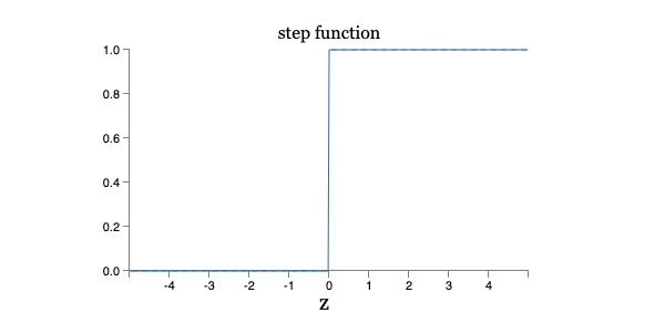
This comparison also explains the relationship between the two neurons: if you replace the sigmoid neuron’s $\sigma$ with a step function, it degenerates into a perceptron, because the output becomes the 0 or 1 you get from passing $w \cdot x + b$ through the step function.

And the reason smoothness matters is that it makes the ideal property from earlier actually hold: after a small adjustment to the parameters (weights and biases), the output really does change by only a small amount.

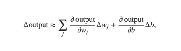
The figure above expresses how a sigmoid neuron’s change in output ($\Delta \text{output}$) arises from changes in its parameters ($\Delta w$ and $\Delta b$). $\Delta w$ is the change in the weight and $\Delta b$ the change in the bias, and the two are not simply added together — each is first multiplied by a partial derivative.

Put even more plainly, you can read the equation above as a simple linear function: $\Delta w$ times one constant, plus $\Delta b$ times another constant, equals $\Delta \text{output}$. Because it is linear, when $\Delta w$ and $\Delta b$ change by only small amounts, $\Delta \text{output}$ naturally changes by only a small amount too. This is exactly what a perceptron cannot do and a sigmoid neuron can.

7 How to Interpret a Sigmoid Neuron’s Output

A sigmoid neuron’s output is no longer just 0 or 1, but any number between 0 and 1 — perhaps 0.2123, 0.5698 or 0.9652. That raises a new question: how should this number be read?

Suppose we use a sigmoid neuron to judge handwritten-digit images. We feed in “image 9” and want the output to tell us whether the image “is the digit 9” or “is not the digit 9”. But the output no longer maps 0 and 1 directly onto False and True the way a perceptron’s did.

The practical approach is to treat the output as a probability. A sigmoid neuron’s output always falls between 0 and 1, which fits the properties of a probability nicely, so it’s very intuitive to take 0.5 as the classification threshold: an output of 0.6 is greater than 0.5, meaning it thinks the image “is the digit 9”; an output of 0.4 is less than 0.5, meaning it thinks it “is not the digit 9”.

8 Conclusion

This article introduced the neuron that is much closer to what modern neural networks use: the sigmoid neuron. Its structure is almost copied from the perceptron, the difference being that both inputs and outputs become continuous values between 0 and 1, with one extra layer — a sigmoid function — applied at the end.

The key is the sigmoid function’s “smoothness”: it ensures that a small tweak to the parameters produces only a small change in the output, avoiding the perceptron’s predicament where an output flips outright and pulls the whole network with it. Only then can learning accumulate step by step. The continuous output brings an extra benefit too — it can be read directly as a probability, using 0.5 as a classification threshold.

Both this article and the previous one, “Understanding the Perceptron”, focus on a single artificial neuron. The next article zooms out to introduce the artificial neural network, and what happens once these neurons are wired together.

8.1 References

• Neural networks and deep learning
• Sigmoid function – Wikipedia
• Partial Differentiation Tutorial