CIFAR-10 in PyTorch: Why Transfer Learning Wins in Just 5 Epochs

1 Introduction

A lot of people who are new to machine learning want to build skills through Kaggle competitions, but get stuck on the very first step: which competition should you even start with? This article’s answer is CIFAR-10 – Object Recognition in Images — the task is simple and the data is clean, which makes it a good choice for your very first Kaggle competition.

The article starts from the competition’s rules, then walks through data preprocessing, building the model, and the training loop, before finishing with a comparison of four models’ training results: a bare-bones CNN, a version with Dropout added, a version that swaps in BatchNorm, and a DenseNet fine-tuned with transfer learning.

The implementation is written in PyTorch — if you’ve never touched it before, it’s worth going through the official tutorial first before coming back here. If you’re coming from TensorFlow or Keras, the code here shouldn’t be hard to follow either. The full code is available on the author’s GitHub.

2 Competition Overview

CIFAR-10 is a well-known dataset in computer vision, and plenty of machine learning beginners use it to practice. CIFAR-10 contains 60,000 32×32 color images, each containing a single object belonging to one of 10 categories. Overall, each category has 6,000 images.

In this competition’s dataset, the organizers have already split the CIFAR-10 dataset into a training set and a test set: the training set has 50,000 images, and the test set has 10,000 images. Each image belongs to one of these 10 categories:

• airplane
• automobile
• bird
• cat
• deer
• dog
• frog
• horse
• ship
• truck

The goal is to build a model that, after training on the 50,000 training images, makes accurate predictions on the remaining 10,000 test images. There’s an interesting design choice here: to stop participants from cheating (by manually labeling the 10,000 test images), the organizers mixed in an extra 290,000 images, so participants have no way of knowing which images are the “real” test set. That means a large chunk of the predictions in the file you submit are actually just noise that isn’t scored at all.

From this overview, it’s clear this is a classic “image classification” task, and each image only ever has one label. There aren’t many categories (10), and the amount of training data per category is very consistent, so there’s no imbalanced-data headache to deal with separately. For a beginner, that means you can put your attention on the model itself instead of spending most of your time cleaning data.

3 Step 1: Importing the Libraries

With the competition’s goal clear, it’s time to get started. First, import the necessary libraries:

# model
import torch
import torch.nn as nn
import torch.nn.functional as F
import torch.optim as optim
from torchvision import models

# dataset
import math
import glob
import pandas as pd
from PIL import Image
from sklearn.model_selection import train_test_split
from torchvision import transforms
from torch.utils.data import Dataset, Subset, DataLoader
import matplotlib.pyplot as plt

# save result
import pickle

Next, let PyTorch grab whatever GPU resources are available on the machine:

torch.manual_seed(2022)
try:
    device = torch.device("mps")
except:
    device = torch.device("cuda") if torch.cuda.is_available() else torch.device("cpu")

This first tries to grab an MPS device — the GPU on Apple Silicon (the author has a separate article covering how to get PyTorch to use a Mac M1’s GPU); if that fails, it falls back to CUDA, and if that also fails, it falls back to the CPU. If you’re running this on a regular NVIDIA machine or on Colab, you’ll simply go down the cuda path.

4 Step 2: Loading the Dataset

Since the author did this project in Colab, the whole project was first uploaded to Google Drive, then the Drive was mounted into Colab, and the training and test data were unzipped:

from google.colab import drive
drive.mount('/gdrive')
!unzip "/gdrive/MyDrive/Colab Notebooks/Kaggle/CIFAR-10 - Object Recognition in Images/cifar-10.zip"
!7z x train.7z
!7z x test.7z

The competition’s raw files come in .7z format, so after unzipping the outer zip file you need to run 7z again to get the actual PNG images. Once that’s done, save the paths to all the training images:

img_names = glob.glob(f"cifar-10/train/*.png")

5 Step 3: Preprocessing the Image Data

Before feeding images into a model, it’s common to do some preprocessing so the model trains more easily and learns better. This project does only the most basic one: normalization. Normalization needs a mean and a standard deviation to work with, and those numbers aren’t picked arbitrarily — they’re computed from the training data itself, separately for each channel (an RGB image has 3 channels).

First, read every image and convert it into a PyTorch tensor:

imgs = []

transform = transforms.Compose([
    transforms.ToTensor(),
])

for img in img_names:
    img = Image.open(img)
    imgs.append(transform(img))

Then, compute the mean and standard deviation for each channel:

imgs = torch.stack(imgs, dim=3)
channel_mean = imgs.view(3, -1).mean(dim=1)
channel_std = imgs.view(3, -1).std(dim=1)
print(f"channel mean: {channel_mean}")
print(f"channel std: {channel_std}")

These two numbers can then go straight into transforms.Compose(), which bundles multiple preprocessing steps into a single pipeline:

transform_fn = transforms.Compose([
    transforms.ToTensor(),
    transforms.Normalize(
        mean=channel_mean,
        std=channel_std
    )
])

Finally, define a PyTorch Dataset. This one needs to handle both training and test scenarios, and the difference comes down to whether csv_path is given: with a label file, it builds a “filename → class index” lookup from the CSV; without one, every label is simply filled in as -1:

class CIFARDataset(Dataset):

    def __init__(self, img_path, transform, csv_path):
        self.csv_path = csv_path
        self.transform = transform

        if csv_path:
            self.img_names = glob.glob(f"{img_path}/*.png")
        else:
            self.img_names = [f"{img_path}/{idx}.png" for idx in range(1, 300001)]

        if csv_path:
            label_df = pd.read_csv(csv_path)
            self.label_idx2name = label_df['label'].unique()
            self.label_name2idx = {}

            for i in range(len(self.label_idx2name)):
                self.label_name2idx[self.label_idx2name[i]] = i
            self.img2label = {}
            for_, row in label_df.iterrows():
                self.img2label[f"{img_path}/{row['id']}.png"] = self.label_name2idx[row['label']]

    def __len__(self):
        return len(self.img_names)

    def __getitem__(self, index):
        img = self.img_names[index]

        if self.csv_path:
            label = self.img2label[img]
            label = torch.tensor(label)
        else:
            label = -1

        img = Image.open(img)
        img = self.transform(img)
        return (img, label)

dataset = CIFARDataset(
    img_path="cifar-10/train",
    transform=transform_fn,
    csv_path="cifar-10/trainLabels.csv",
)

To evaluate the model, the training set gets split further into a training portion and a validation portion. The reason for carving out a validation split is that Kaggle’s test set has no labels, so there’s no way to know locally how well the model is doing — this held-out split is the only “mock exam” available:

indexes = list(range(len(dataset)))
train_indexes, valid_indexes = train_test_split(indexes, test_size=0.2)
train_dataset = Subset(dataset, train_indexes)
valid_dataset = Subset(dataset, valid_indexes)

print(f"number of samples in train_dataset: {len(train_dataset)}")
print(f"number of samples in valid_dataset: {len(valid_dataset)}")

And build a PyTorch DataLoader for each:

train_dataloader = DataLoader(
    train_dataset,
    batch_size=32,
    shuffle=True
)

valid_dataloader = DataLoader(
    valid_dataset,
    batch_size=32,
    shuffle=True
)

Defining your own Dataset and DataLoader in PyTorch is common practice — if you’re not familiar with it, the official tutorial is a good reference.

With the DataLoader in hand, you can pull out a batch and plot a few images to sanity-check them. There are two easy-to-miss gotchas here: first, the images have already been normalized, so plotting them directly will make the colors look completely off — you need to undo the normalization first; second, Matplotlib expects the “channel” dimension last, while a PyTorch tensor puts it first, so permute() is needed to reorder the dimensions:

def show_samples(batch_img, batch_label=None, num_samples=16):

    sample_idx = 0
    total_col = 4
    total_row = math.ceil(num_samples / 4)
    col_idx = 0
    row_idx = 0

    fig, axs = plt.subplots(total_row, total_col, figsize=(15, 15))

    while sample_idx < num_samples:
        img = batch_img[sample_idx]
        img = img.view(3, -1) * channel_std.view(3, -1) + channel_mean.view(3, -1)
        img = img.view(3, 224, 224)
        img = img.permute(1, 2, 0)
        axs[row_idx, col_idx].imshow(img)

        if batch_label != None:
            axs[row_idx, col_idx].set_title(dataset.label_idx2name[(batch_label[sample_idx])])
        
        sample_idx += 1
        col_idx += 1
        if col_idx == 4:
            col_idx = 0
            row_idx += 1

batch_img, batch_label = next(iter(train_dataloader))

show_samples(batch_img, batch_label, 16)

6 Step 4: Building the Model (VallinaCNN)

Start with the simplest, most bare-bones model for this image classification task. It has only three convolution layers followed by one linear layer, and is named VallinaCNN in the code (kept as-is here):

class VallinaCNN(nn.Module):

    def  __init__(self):
        super(VallinaCNN, self).__init__()

        self.conv1 = nn.Conv2d(in_channels=3, out_channels=16, kernel_size=3, padding=1)
        self.conv2 = nn.Conv2d(in_channels=16, out_channels=32, kernel_size=3, padding=1)
        self.conv3 = nn.Conv2d(in_channels=32, out_channels=64, kernel_size=3, padding=1)
        self.linear1 = nn.Linear(64*8*8, 10)


    def forward(self, inp):
        x = F.relu(self.conv1(inp))
        x = F.max_pool2d(x, (2, 2))
        x = F.relu(self.conv2(x))
        x = F.max_pool2d(x, (2, 2))
        x = F.relu(self.conv3(x))
        x = torch.flatten(x, 1)
        out = self.linear1(x)

        return out

The structure is simple: convolutions extract features, max pooling shrinks the spatial size, and after repeating this a few times the features get flattened and handed to the final linear layer, which outputs a score for each of the 10 classes. After building the model, print out the parameter count — it’ll be useful later when comparing against the other models:

net = VallinaCNN()
net.to(device)
print(f"number of paramaters: {sum([param.numel() for param in net.parameters() if param.requires_grad])}")

7 Step 5: Loss Function and Optimizer

Since this is a multi-class classification problem, CrossEntropyLoss() is the loss function, and SGD is used to update the model’s parameters:

criterion = nn.CrossEntropyLoss()
optimizer = optim.SGD(net.parameters(), lr=0.005)

8 Step 6: Training & Validation Loop

The training and validation loops share almost the same skeleton: each round pulls a batch of data from the DataLoader, feeds it into the model, and gets the output. The difference is that train() calls loss.backward() and optimizer.step() to update the model’s parameters, while validate() only computes accuracy and loss without touching the model.

First, a small helper for computing accuracy: run the model’s output through softmax once, take the class with the highest probability, and compare it against the true label:

def get_accuracy(output, label):
    output = output.to("cpu")
    label = label.to("cpu")

    sm = F.softmax(output, dim=1)
    _, index = torch.max(sm, dim=1)
    return torch.sum((label == index)) / label.size()[0]

Next, train(). It prints the average loss every 500 batches, so you can watch the numbers trend downward during training:

def train(model, dataloader):
    model.train()
    running_loss = 0.0
    total_loss = 0.0
    running_acc = 0.0
    total_acc = 0.0

    for batch_idx, (batch_img, batch_label) in enumerate(dataloader):
        batch_img = batch_img.to(device)
        batch_label = batch_label.to(device)

        optimizer.zero_grad()
        output = net(batch_img)
        loss = criterion(output, batch_label)
        loss.backward()
        optimizer.step()

        running_loss += loss.item()
        total_loss += loss.item()

        acc = get_accuracy(output, batch_label)
        running_acc += acc
        total_acc += acc
        
        if batch_idx % 500 == 0 and batch_idx != 0:
            print(f"[step: {batch_idx:4d}] loss: {running_loss / 500:.3f}")
            running_loss = 0.0
            running_acc = 0.0
    return total_loss / len(dataloader), total_acc / len(dataloader)

validate() is the same, except the three lines that update the parameters are commented out:

def validate(model, dataloader):
    model.eval()
    total_loss = 0.0
    total_acc = 0.0

    for batch_idx, (batch_img, batch_label) in enumerate(dataloader):

        batch_img = batch_img.to(device)
        batch_label = batch_label.to(device)

        # optimizer.zero_grad()
        output = net(batch_img)
        loss = criterion(output, batch_label)
        # loss.backward()
        # optimizer.step()

        total_loss += loss.item()
        acc = get_accuracy(output, batch_label)
        total_acc += acc

    return total_loss / len(dataloader), total_acc / len(dataloader)

9 Step 7: Training the Model

The main loop runs for 20 epochs, running one train and one validate each epoch and recording the loss. The final if statement is the key part: the model is only saved to disk when the validation loss hits a new low, so whatever is left on disk after training is the best-performing set of parameters, not just the parameters from the last epoch:

EPOCHS = 20
train_history = []
valid_history = []

for epoch in range(EPOCHS):
    train_loss, train_acc = train(net, train_dataloader)
    valid_loss, valid_acc = validate(net, valid_dataloader)
    print(f"Epoch: {epoch:2d}, training loss: {train_loss:.3f}, training acc: {train_acc:.3f} validation loss: {valid_loss:.3f}, validation acc: {valid_acc:.3f}")

    train_history.append(train_loss)
    valid_history.append(valid_loss)

    if valid_loss <= min(valid_history):
        torch.save(net.state_dict(), "net.pt")

10 Step 8: VallinaCNN Training Results

Once training finishes, plotting how training loss and validation loss changed over time shows how well it actually trained.

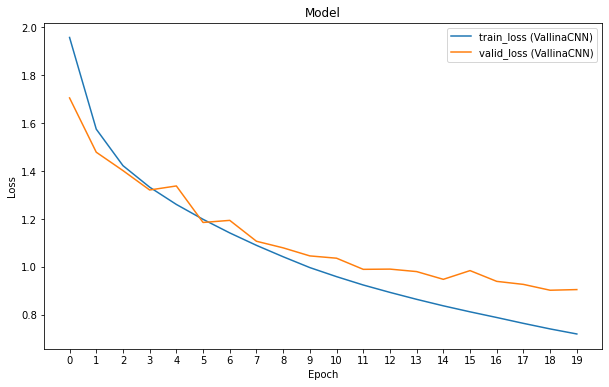
The chart above shows VallinaCNN’s training results. Both training loss and validation loss keep dropping at first, but starting around epoch 8, the validation loss’s rate of decline starts to slow down. By epoch 19, there’s already a visible gap between validation loss and training loss.

This is a problem commonly seen when training neural networks: overfitting. In plain terms, the model has memorized the training data and struggles on data it hasn’t seen before. Two curves pulling further and further apart is the textbook symptom.

11 Step 9: Adding Dropout to the Model (CNNDropout)

There are many ways to ease overfitting, and one of the simplest is adding a dropout layer — this site also has a dedicated article walking through why and how dropout works if you want the fuller picture:

class CNNDropout(nn.Module):

    def __init__(self):
        super(CNNDropout, self).__init__()

        self.conv1 = nn.Conv2d(in_channels=3, out_channels=16, kernel_size=3, padding=1)
        self.conv1_dropout = nn.Dropout(p=0.4)
        self.conv2 = nn.Conv2d(in_channels=16, out_channels=32, kernel_size=3, padding=1)
        self.conv2_dropout = nn.Dropout(p=0.4)
        self.conv3 = nn.Conv2d(in_channels=32, out_channels=64, kernel_size=3, padding=1)
        self.linear1 = nn.Linear(64*8*8, 10)


    def forward(self, inp):
        x = F.relu(self.conv1(inp))
        x = F.max_pool2d(x, (2, 2))
        x = self.conv1_dropout(x)

        x = F.relu(self.conv2(x))
        x = F.max_pool2d(x, (2, 2))
        x = self.conv2_dropout(x)

        x = F.relu(self.conv3(x))
        x = torch.flatten(x, 1)
        out = self.linear1(x)

        return out

CNNDropout is similar to VallinaCNN, except the output of each max-pooling step also passes through a dropout layer. After training it for the same 20 epochs, compare its results against the original VallinaCNN:

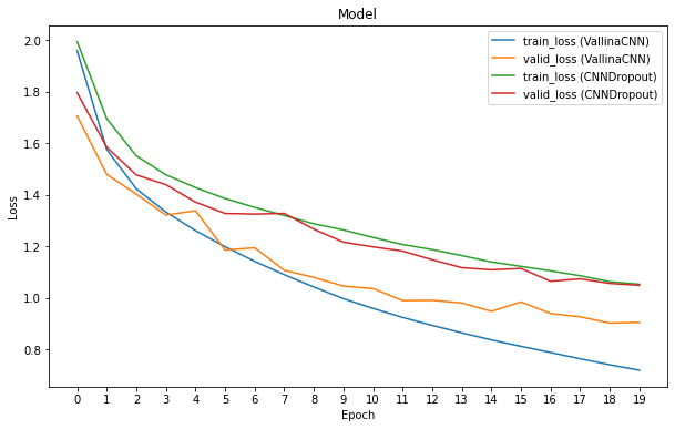
The original overfitting problem is indeed reduced — even at epoch 19, validation loss is still trending down along with training loss. However, compared with VallinaCNN (which has no dropout), CNNDropout’s training loss and validation loss are both still noticeably higher. In other words, overfitting was suppressed, but overall predictive performance didn’t actually improve.

12 Step 10: Replacing Dropout with BatchNorm (CNNBatchNorm)

In practice, BatchNorm is often used in place of Dropout — on top of also reducing overfitting, it can speed up training:

class CNNBatchNorm(nn.Module):

    def __init__(self):
        super(CNNBatchNorm, self).__init__()

        self.conv1 = nn.Conv2d(in_channels=3, out_channels=16, kernel_size=3, padding=1)
        self.conv1_bn = nn.BatchNorm2d(num_features=16)
        self.conv2 = nn.Conv2d(in_channels=16, out_channels=32, kernel_size=3, padding=1)
        self.conv2_bn = nn.BatchNorm2d(num_features=32)
        self.conv3 = nn.Conv2d(in_channels=32, out_channels=64, kernel_size=3, padding=1)
        self.conv3_bn = nn.BatchNorm2d(num_features=64)
        self.linear1 = nn.Linear(64*8*8, 10)

    def forward(self, inp):
        x = self.conv1(inp)
        x = self.conv1_bn(x)
        x = F.relu(x)
        x = F.max_pool2d(x, (2, 2))

        x = self.conv2(x)
        x = self.conv2_bn(x)
        x = F.relu(x)
        x = F.max_pool2d(x, (2, 2))

        x = self.conv3(x)
        x = self.conv3_bn(x)
        x = F.relu(x)

        x = torch.flatten(x, 1)
        out = self.linear1(x)

        return out

Note where BatchNorm sits: right after each convolution layer, and before the ReLU. After training this for 20 epochs, compare its results against both VallinaCNN and CNNDropout:

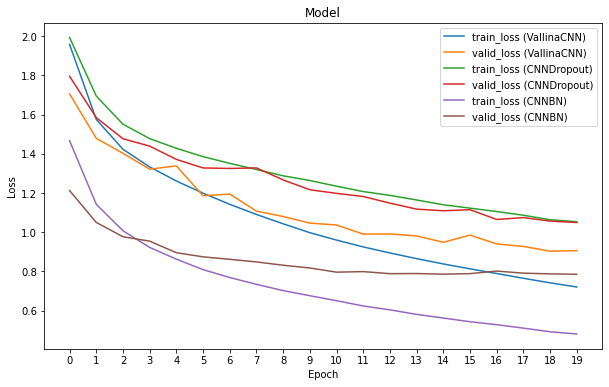
The chart shows that, after the same 20 epochs, CNNBatchNorm’s training loss and validation loss are both clearly lower than VallinaCNN’s and CNNDropout’s. CNNBatchNorm also dramatically shortens the time needed to train: after just 4 epochs, its training and validation loss are already lower than the other two models ever reach. That’s “faster training” in its most direct form: the same result in a fifth of the time.

13 Step 11: Improving Accuracy with Transfer Learning (PretrainDenseNet)

So far, three models have been tried — VallinaCNN, CNNDropout, and CNNBatchNorm — and each shows how a given technique affects the model’s performance. Back to the original question: what does it actually take to train a good enough model for this Kaggle competition? The answer is transfer learning.

The idea behind transfer learning is not to train from scratch, but to take a model that’s already been trained on a large amount of data and fine-tune it. Here, DenseNet is loaded from PyTorch’s TorchVision Models, along with the weights it learned on ImageNet. ImageNet has 1,000 classes, and this task only needs 10, so the model’s classifier head needs to be swapped out:

class PretrainDenseNet(nn.Module):

    def __init__(self):
        super(PretrainDenseNet, self).__init__()
        model = models.densenet121(pretrained=True)
        num_classifier_feature = model.classifier.in_features
        model.classifier = nn.Sequential(
            nn.Linear(num_classifier_feature, 256),
            nn.ReLU(),
            nn.Dropout(0.3),
            nn.Linear(256, 10)
        )       
        self.model = model

        # for param in self.model.named_parameters():
            # if 'features' in param[0]:
            # param[1].requires_grad = False

    def forward(self, x):
        return self.model(x)

(The pretrained=True argument here is how this was written at the time — newer versions of TorchVision use a weights= argument instead.)

In transfer learning, the usual approach is to freeze the parameters of the model’s main body and only train the new classifier head — that’s what the commented-out lines above would do. In this project, though, the whole model was left trainable, and it still performed well:

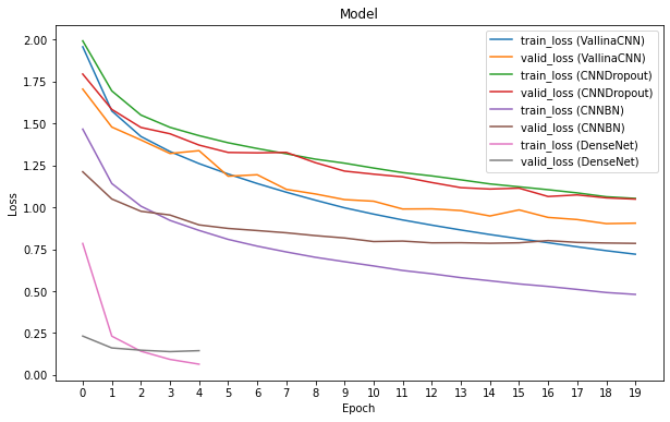
The chart shows that after training for only 5 epochs, both training loss and validation loss are already close to 0. Placed next to the previous three models, which each needed the full 20 epochs, the gap is striking.

14 Conclusion

This article walked through Kaggle’s CIFAR-10 – Object Recognition in Images competition — a clean task with balanced classes that makes it a great fit for a beginner’s first competition.

Along the way, using the same data and the same training loop, it compared how a plain CNN, Dropout, and BatchNorm affect model performance: Dropout suppresses overfitting but leaves overall loss on the high side, while BatchNorm does both — controlling overfitting and speeding up convergence — at once. Transfer learning then pulled the results further ahead, showing that even with limited hardware and limited training data, standing on the shoulders of an already-trained model can still get you a high-performing model.

This article doesn’t cover how to generate the submission.csv Kaggle expects — for that part of the code, see the author’s GitHub.