Parallel Programming by Example: Split, Compute, Reduce

1 Introduction

The previous article, What Is Parallel Programming?, covered the basic concept. This one goes one level deeper: using a very simple example program, we’ll see exactly how an originally single-threaded program gets split apart and handed off to multiple cores.

The article has three parts: first, why parallelizing isn’t just an option anymore but a necessity; then a complete walkthrough of parallelizing an array-sum program, reduction included; and finally a summary of the two directions parallelization can take and the three elements you always have to consider.

2 Why Parallel Programming Is No Longer Optional

The previous article talked about why we’d want parallel programming. Here we’re after something harder: why, today, parallelizing is a step you basically can’t skip.

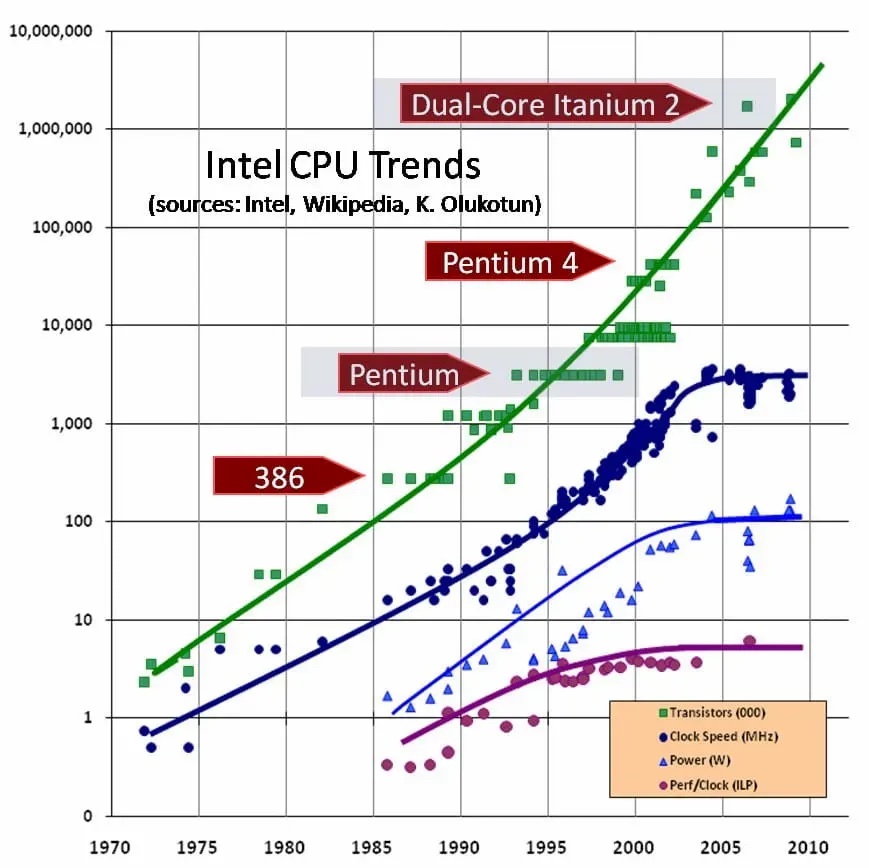
As the chart above shows, the four lines from top to bottom represent transistor count, clock speed, power, and ILP. Following Moore’s Law, transistor count (green) keeps climbing year over year — but a single CPU’s clock speed (dark blue) has flattened out, and so has ILP (purple).

ILP stands for Instruction-Level Parallelism: even on a single core, the compiler and the CPU architecture can still parallelize at the instruction level to speed up execution. In other words, this is the part where hardware and the compiler quietly parallelize things for you — no extra work required from the engineer.

That’s exactly where the problem sits. A single core’s clock speed and ILP have both run into a wall — the free performance has mostly already been claimed. The dividend from more transistors now arrives as “more cores,” not “one faster core.” If you want a program to keep getting faster, you have to go back to the software itself and write it to actually make use of multiple cores.

3 A Simple Parallel Programming Example

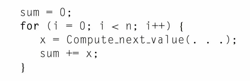
Say we have an array with n elements, none of them depending on each other, and we want to run some computation on every element and sum up the results. The program above does exactly that: one pass through a loop, one element at a time, all handled by a single core.

The key detail here is “no dependency between elements.” Element 5’s result has no effect on how element 6 gets computed, so it doesn’t matter which one gets computed first — that’s the signal that something can be parallelized.

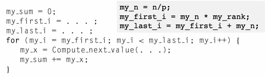
Because the elements have no dependencies, we can use parallel programming techniques to divide all of the array’s elements evenly across every core. Each core only needs to know two things: which range it’s responsible for, and where to put its own partial result (the my_sum variable in the diagram).

For example, say the computer currently has p cores and the array has n elements — we can evenly hand out n/p elements to each core. What used to be one core carrying all n elements is now shared across multiple cores, so the run time naturally shrinks.

Real numbers make this easier to picture. As shown above, say the array has 24 numbers and the computer has 8 cores — we’d hand out 3 numbers to each core.

Every core computes its own result and stores it in a my_sum variable. Finally, one master core is responsible for summing up every core’s result. Thanks to parallel programming, the 24-number computation that used to fall entirely on the master core is now handled by 8 cores working on their own slice at the same time, with the master core just pulling everyone’s results together at the end.

4 Parallelizing the Reduction Step

In the example above, the master core is the one that finally sums up every core’s result — in other words, it takes the 8 numbers and merges them down into 1. This process of going from “many elements” to “few elements” through computation is called reduction.

Reduction itself can usually be parallelized too, and this step is easy to overlook: if this final cleanup is still left entirely to the master core, it eats back some of the time saved by splitting the work up front.

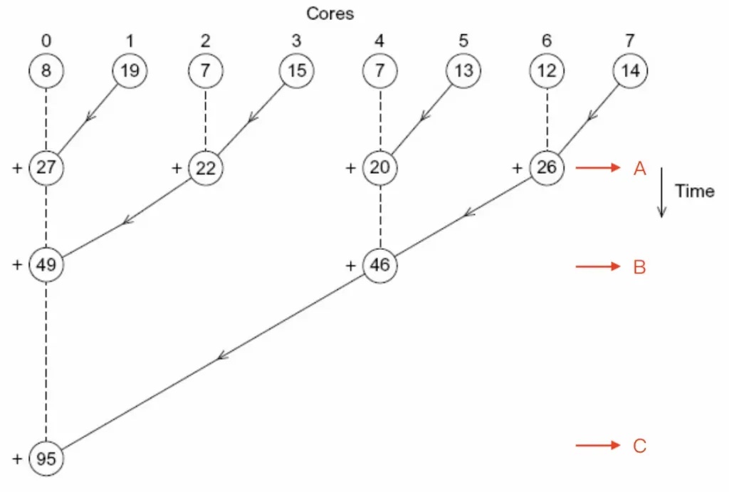
The approach is to pair things up: core 0 adds core 1’s result, core 2 adds core 3’s, core 4 adds core 5’s, core 6 adds core 7’s. That means at time point A, 4 additions happen at once. Then the remaining 4 numbers pair up again, then 2, and it converges down to a single number.

After rewriting the reduction step with parallel programming, what used to be 7 additions on the master core (core 0) is now just 3.

5 Two Directions for Parallelizing a Program

When parallelizing an originally single-threaded program, there are two directions you can take: task parallelism and data parallelism.

• Task parallelism

Split the original problem into several different tasks, with each core handling its own task. For example, say a bakery has 3 bakers making 300 cakes, and each baker is responsible for a different step of every cake — so what each baker actually does is different from the others.

• Data parallelism

Split the data-processing part of the problem so each core handles a portion of the data. In the same bakery example, each baker would instead be responsible for 100 whole cakes — so what each baker does is identical, just applied to different cakes.

The array-sum example above is standard data parallelism: every core runs the exact same computation, just on different data.

6 Three Elements to Consider When Parallelizing

When parallelizing an originally single-threaded program, there are three elements you need to account for: communication, load balancing, and synchronization.

• Communication

A parallel program typically involves multiple cores, and those cores need some way to pass information to each other. In the example above, every core’s my_sum eventually has to make its way to the master core — that’s a form of communication.

• Load balancing

How do you make sure every core is carrying a roughly even share of the work? In the example above, we split the data evenly by count. But sometimes different pieces of data take different amounts of time to process, and dividing purely by count can leave some cores still grinding away while others sit idle.

• Synchronization

Sometimes one core needs to wait for another to finish before it can continue. In the reduction example, core 0 has to wait until core 1 has actually finished computing its my_sum before the combined result is correct.

Of these three, communication and synchronization exist to make sure the parallel program produces the same result as the original serial program; load balancing exists to optimize the parallel program’s performance.

7 Conclusion

This article started from hardware trends to explain why parallel programming is “necessary” today: clock speed and ILP have both stalled, so performance growth can only come from more cores. It then walked through an array-sum example end to end — splitting the data, computing independently, and converging the results back with reduction.

Finally, it laid out the two directions parallelization can take (task parallelism and data parallelism) and the three elements you always have to watch (communication, load balancing, and synchronization). Those three elements keep showing up again when we get to the Shared Memory Model and the Distributed Memory Model — worth keeping in the back of your mind.