Building an Image Classifier with PyTorch's ResNet

1 Introduction

What this article does is simple: use PyTorch’s TorchVision library to load a model that is already trained, and use it directly for inference — no training of our own involved.

The problem we’re solving is “image classification,” so we’ll load a Residual Neural Network (ResNet) from TorchVision, feed it a few pictures of our own choosing, and see whether it gets them right. The whole flow goes from loading the model, defining the image preprocessing, and feeding in images, all the way to translating the model’s numeric output back into human-readable class names.

Before reading on, it helps to already have a basic sense of “model training” and “model inference” in machine learning — this site has dedicated articles on both. If you’d like to go a step further and understand how a neural network classifies images in the first place, the “How Does a Neural Network Classify Images” article is also worth a look.

The full code is available on Colab and GitHub, so you can follow along and run it yourself.

2 Importing the Libraries

TorchVision ships with plenty of open-source models, and many of them have already been trained on the ImageNet dataset. That means we don’t need to train a model from scratch — we can load an already-trained model directly and experience what “model inference” feels like.

The value here is really about cost: ImageNet has over a million labeled images, and training a model from zero would burn through a huge amount of GPU time. Loading someone else’s already-trained weights, by contrast, takes just one line of code.

First, let’s import the libraries this small project will use:

import torch
from torchvision import models
from torchvision import transforms

import json
from PIL import Image

3 Checking Which Models TorchVision Offers

To see what models TorchVision actually provides, just call dir() on the models module to list everything under it:

dir(models)

Output:

['AlexNet',
'ConvNeXt',
'DenseNet',
'EfficientNet',
'GoogLeNet',
'GoogLeNetOutputs',
'Inception3',
'InceptionOutputs',
'MNASNet',
'MobileNetV2',
'MobileNetV3',
'RegNet',
'ResNet',
'ShuffleNetV2',
'SqueezeNet',
'VGG',
'VisionTransformer',
'_GoogLeNetOutputs',
...
'resnet',
'resnet101',
'resnet152',
'resnet18',
'resnet34',
'resnet50',
'resnext101_32x8d',
'resnext50_32x4d',
'segmentation',
'shufflenet_v2_x0_5',
'shufflenet_v2_x1_0',
'shufflenet_v2_x1_5',
'shufflenet_v2_x2_0',
'shufflenetv2',
'squeezenet',
'squeezenet1_0',
'squeezenet1_1',
'vgg',
'vgg11',
'vgg11_bn',
'vgg13',
'vgg13_bn',
'vgg16',
'vgg16_bn',
'vgg19',
...]

Looking at this output, some names are capitalized and some are lowercase.

Capitalized names are Python classes; lowercase names are Python functions. For example, we could build a ResNet model directly using the ResNet class.

But if we want a specific, off-the-shelf ResNet variant — say, a 101-layer ResNet — we can just call the resnet101 function; for an 18-layer ResNet, resnet18. In other words, the number after resnet in the function name is the number of layers in the network. More layers generally means a bigger model, usually with better accuracy, but slower inference.

4 Loading a Pretrained ResNet Model

When loading the ResNet model from TorchVision, we also set pretrained to True, to make sure the model’s parameters have already been trained (in newer versions of TorchVision, pretrained has been replaced by a weights argument, but the idea is the same):

resnet = models.resnet101(pretrained=True, progress=True)

progress=True just shows a progress bar while the weights are downloading — the first run will take a moment.

Let’s print out ResNet’s model architecture:

resnet

ResNet(
(conv1): Conv2d(3, 64, kernel_size=(7, 7), stride=(2, 2), padding=(3, 3), bias=False)
(bn1): BatchNorm2d(64, eps=1e-05, momentum=0.1, affine=True, track_running_stats=True)
(relu): ReLU(inplace=True)
(maxpool): MaxPool2d(kernel_size=3, stride=2, padding=1, dilation=1, ceil_mode=False)
(layer1): Sequential(
    (0): Bottleneck(
        (conv1): Conv2d(64, 64, kernel_size=(1, 1), stride=(1, 1), bias=False)
        (bn1): BatchNorm2d(64, eps=1e-05, momentum=0.1, affine=True, track_running_stats=True)
        (conv2): Conv2d(64, 64, kernel_size=(3, 3), stride=(1, 1), padding=(1, 1), bias=False)
        (bn2): BatchNorm2d(64, eps=1e-05, momentum=0.1, affine=True, track_running_stats=True)
        (conv3): Conv2d(64, 256, kernel_size=(1, 1), stride=(1, 1), bias=False)
        (bn3): BatchNorm2d(256, eps=1e-05, momentum=0.1, affine=True, track_running_stats=True)
        (relu): ReLU(inplace=True)
        (downsample): Sequential(
            (0): Conv2d(64, 256, kernel_size=(1, 1), stride=(1, 1), bias=False)
            (1): BatchNorm2d(256, eps=1e-05, momentum=0.1, affine=True, track_running_stats=True)
        )
    )
    (1): Bottleneck(
        (conv1): Conv2d(256, 64, kernel_size=(1, 1), stride=(1, 1), bias=False)
        (bn1): BatchNorm2d(64, eps=1e-05, momentum=0.1, affine=True, track_running_stats=True)
        (conv2): Conv2d(64, 64, kernel_size=(3, 3), stride=(1, 1), padding=(1, 1), bias=False)
        (bn2): BatchNorm2d(64, eps=1e-05, momentum=0.1, affine=True, track_running_stats=True)
        (conv3): Conv2d(64, 256, kernel_size=(1, 1), stride=(1, 1), bias=False)
        (bn3): BatchNorm2d(256, eps=1e-05, momentum=0.1, affine=True, track_running_stats=True)
        (relu): ReLU(inplace=True)
    )
...
)
...
(avgpool): AdaptiveAvgPool2d(output_size=(1, 1))
(fc): Linear(in_features=2048, out_features=1000, bias=True)
)

Even from this truncated printout, you can tell ResNet is a pretty “deep” model. Part of why ResNet is so well known is that it introduced techniques that make very deep networks much easier to train.

Look closely at ResNet’s last layer: it’s a Linear layer with an output vector of length 1000. That means for every image we feed into ResNet, it returns a 1000-dimensional vector (1000 numbers), where each number is a score for how likely the image belongs to that particular class. That 1000 isn’t an arbitrary choice — it’s the number of classes defined by the ImageNet dataset, and we’ll run into it again later when we process the output.

Next, let’s count how many parameters ResNet has:

sum([param.numel() for param in resnet.parameters()])

It turns out ResNet has as many as 44.54 million parameters! But since all of them were already trained on the ImageNet dataset, that’s one big headache we get to skip.

5 Defining the Image Preprocessing

Before we can actually feed an image into ResNet, we need to preprocess it first. In other words, we can’t just grab any random picture and throw it straight into the ResNet model — the input image needs to match ResNet’s expected format to get the best predictions.

The reasoning is straightforward: the model was originally trained on images processed into a specific, fixed format. If we feed it images in a different format at inference time, the value distribution the model sees no longer matches what it saw during training, and the results end up skewed.

We can use TorchVision’s transforms to preprocess our images:

preprocess = transforms.Compose([
    transforms.Resize(256),
    transforms.CenterCrop(224),
    transforms.ToTensor(),
    transforms.Normalize(
        mean=[0.485, 0.456, 0.406],
        std=[0.229, 0.224, 0.225]
    )
])

In the transforms.Compose above, we’ve defined the following preprocessing steps:

• transforms.Resize(256): resize the image to 256 × 256
• transforms.CenterCrop(224): crop the image to 224 × 224
• transforms.ToTensor(): convert the image into a PyTorch Tensor
• transforms.Normalize: normalize every channel of the image

Compose simply means “chain these steps into one pipeline” — calling preprocess(img) once runs all four steps above in sequence. As for the mean and std values passed to Normalize, those are the ImageNet dataset’s per-channel statistics across the RGB channels — you can just reuse them as-is.

Before feeding an image into ResNet, we’ll always run it through this preprocessing pipeline first, and only then pass the processed image into the model.

6 Downloading & Reading the Images

Next, we need to go find some images we’re interested in online and download them into our working directory.

In our code example, we download three images using curl:

!curl https://www.princeton.edu/sites/default/files/styles/half_2x/public/images/2022/02/KOA_Nassau_2697x1517.jpg?itok=iQEwihUn > dog.jpg
!curl https://images.theconversation.com/files/443350/original/file-20220131-15-1ndq1m6.jpg > cat.jpg
!curl https://static.onecms.io/wp-content/uploads/sites/28/2020/02/brussels-airlines-smurfs-plane-PLANEPAINT0418.jpg > plane.jpg

(The leading ! is Jupyter/Colab syntax, meaning this line should be handed off to the shell rather than run as Python code.)

The three images look like this:

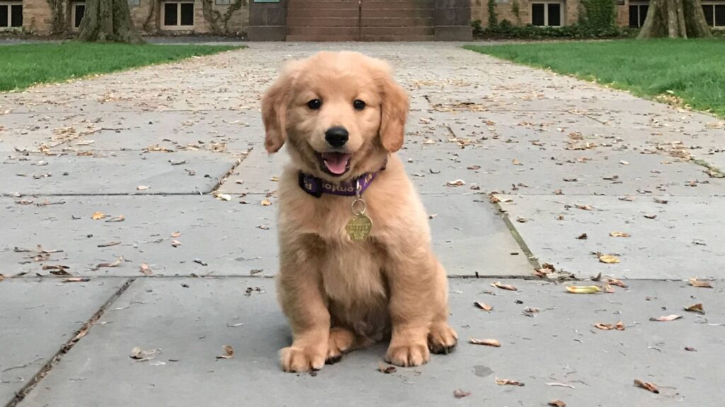
We’re hoping ResNet can correctly classify all three of these images!

Next, let’s use the PIL package to load the three images we just downloaded:

img1 = Image.open("dog.jpg")
img2 = Image.open("cat.jpg")
img3 = Image.open("plane.jpg")

If you’re running this in a Jupyter environment, you can call display directly to show an image:

display(img3)

7 Preprocessing the Images

In this step, we run our images through the preprocess pipeline we defined earlier:

img1 = preprocess(img1)
img2 = preprocess(img2)
img3 = preprocess(img3)

And check their shapes:

print(f"img1 shape: {img1.shape}")
print(f"img2 shape: {img2.shape}")
print(f"img3 shape: {img3.shape}")

You’ll see all three have become 3 × 224 × 224. Three images that originally had different sizes get squeezed into the exact same shape by the same pipeline — that’s exactly what lets us pack them into a single batch next.

8 Feeding the Images into ResNet

Before we run inference, we first need to switch the model into “eval” mode:

resnet.eval()

This line can’t be skipped. Some layers (like BatchNorm and Dropout) behave differently during training versus inference, and eval() is how we tell PyTorch “this is inference, not training.”

We have three images, and we want to feed all three in at once rather than one at a time. So we need to pack them into a single batch:

inp_batch = torch.stack([img1, img2, img3])

torch.stack adds an extra dimension at the front — three 3 × 224 × 224 images become a single 3 × 3 × 224 × 224 tensor, where the leading 3 is the batch size.

Now let’s feed the batch into ResNet:

out_batch = resnet(inp_batch)

Let’s check the shape of ResNet’s output:

out_batch.shape

torch.Size([3, 1000])

This tells us the model outputs a 1000-dimensional vector for each image (1000 numbers), where each number represents the score for that image belonging to a particular class.

9 Interpreting the Model’s Output

At this point, we know the model’s output contains scores for 1000 classes, but we still don’t know what those classes actually are. Since the ResNet we downloaded was pretrained on the ImageNet dataset, its output format follows ImageNet’s own 1000 class definitions.

In other words, the model will only tell you “class #207 has the highest score” — it’s on us to look up what class #207 actually is.

Let’s download ImageNet’s list of 1000 defined classes:

!curl https://raw.githubusercontent.com/xmartlabs/caffeflow/master/examples/imagenet/imagenet-classes.txt > imagenet-classes.txt

Read the contents out of the txt file:

with open("/content/imagenet-classes.txt", 'r') as f:
    labels = [line.strip() for line in f.readlines()]

labels now holds the actual names of all 1000 classes:

labels

['tench, Tinca tinca',
'goldfish, Carassius auratus',
'great white shark, white shark, man-eater, man-eating shark, Carcharodon carcharias',
'tiger shark, Galeocerdo cuvieri',
'hammerhead, hammerhead shark',
'electric ray, crampfish, numbfish, torpedo',
'stingray',
'cock',
'hen',
'ostrich, Struthio camelus',
'brambling, Fringilla montifringilla',
'goldfinch, Carduelis carduelis',
'house finch, linnet, Carpodacus mexicanus',
'junco, snowbird',
'indigo bunting, indigo finch, indigo bird, Passerina cyanea',
'robin, American robin, Turdus migratorius',
'bulbul',
'jay',
'magpie',
'chickadee',
'water ouzel, dipper',
'kite',
'bald eagle, American eagle, Haliaeetus leucocephalus',
'vulture',
'great grey owl, great gray owl, Strix nebulosa',
'European fire salamander, Salamandra salamandra',
'common newt, Triturus vulgaris',
'eft',
'spotted salamander, Ambystoma maculatum',
'axolotl, mud puppy, Ambystoma mexicanum',
'bullfrog, Rana catesbeiana',
'tree frog, tree-frog',
'tailed frog, bell toad, ribbed toad, tailed toad, Ascaphus trui',
'loggerhead, loggerhead turtle, Caretta caretta',
'leatherback turtle, leatherback, leathery turtle, Dermochelys coriacea',
'mud turtle',
'terrapin',
'box turtle, box tortoise',
'banded gecko',
'common iguana, iguana, Iguana iguana',
'American chameleon, anole, Anolis carolinensis',
'whiptail, whiptail lizard',
'agama',
'frilled lizard, Chlamydosaurus kingi',
'alligator lizard',
'Gila monster, Heloderma suspectum',
'green lizard, Lacerta viridis',
'African chameleon, Chamaeleo chamaeleon',
'Komodo dragon, Komodo lizard, dragon lizard, giant lizard, Varanus komodoensis',
'African crocodile, Nile crocodile, Crocodylus niloticus',
'American alligator, Alligator mississipiensis',
'triceratops',
'thunder snake, worm snake, Carphophis amoenus',
'ringneck snake, ring-necked snake, ring snake',
'hognose snake, puff adder, sand viper',
'green snake, grass snake',
'king snake, kingsnake',
...
]

Next, for each image, we want to grab the class with the highest score — the class the model thinks that image belongs to:

_, index = torch.max(out_batch, dim=1)

torch.max returns both the maximum value and its position; here we only care about the position, so we discard the first return value with _. dim=1 means we’re searching for the max along that length-1000 class axis.

index

tensor([207, 281, 404]

index is a tensor with 3 elements: 207 is the class of the first image, 281 the class of the second, and 404 the class of the third.

We can use the labels list we built earlier to turn these numeric classes into their real names:

for idx in index:
    print(labels[idx.item()])

Output:

golden retriever
tabby, tabby cat
airliner

Sure enough, the model correctly classified all three images: the first as a “golden retriever,” the second as a “tabby cat,” and the third as an “airliner.” And the answers are even more specific than we expected — not just “dog,” but “golden retriever”; not just “cat,” but “tabby cat.”

10 Conclusion

In this article, we learned how to load an already-trained ResNet model via TorchVision and run inference with it. The whole flow really comes down to just five steps: load the model, define the preprocessing, read in the images, pack them into a batch and feed them to the model, and map the output index back to a class name.

Beyond image classification, plenty of other AI applications can make good use of models someone else has already trained. Sometimes we simply don’t have access to a large enough dataset, or the resources to train such a large model ourselves — so instead, we can build on top of a model someone else already trained on a massive dataset, and then further train it on our own, smaller dataset.

This dramatically lowers the cost of training a model, and this technique is known as Transfer Learning. When we train a model on our own dataset this way, that dataset usually isn’t very large, and typically only a portion of the model’s parameters get trained — a process also known as Fine-Tuning.

If you’re on an Apple Silicon Mac and would like this same kind of workflow to run with GPU acceleration instead of just the CPU, see Running PyTorch on Apple Silicon: Enabling M1 GPU Training for how to get PyTorch talking to the M1’s GPU.