Dream-RSI: Replay History as a Free Simulator, Not a World Model

1 Introduction
If you’ve ever built an agent system that iterates on its own improvement logic, you’ve probably hit this problem: the improvement logic itself should also get better over time, but figuring out “is this new version actually better” usually means spending real money to run a full round first. That’s exactly the problem Dream-RSI (Tong Zheng et al., a collaboration between Google, University of Maryland, Google DeepMind, and University of Virginia; RSI stands for Recursive Self-Improvement) sets out to solve. When AI agents are used for scientific or algorithmic discovery — think AlphaEvolve-style systems — an exploration policy decides which direction to dig deeper into, when to branch out in parallel, and when to give up on a path. Can that policy improve itself cheaply?
The paper’s answer is refreshingly direct: treat the discovery history that’s already been generated as a replayable database. To test whether a new policy is good, you don’t need to actually re-run any code — let the new policy read the history and ask “what would get revealed if I explored in a different order,” and score it from that alone. This lets you screen thousands of candidate policies at near-zero cost. The mechanism is genuinely clever, and the paper’s own ablation confirms it beats the more common alternative (summarizing history into a text prompt).
But what makes this paper worth your time isn’t only what it does. Honestly, it’s an engineering-solid paper wrapped in an oversold narrative — it frames itself as using a “World Model,” but a genuine world model is a trained function that generalizes to states it has never seen, while Dream-RSI’s simulator only replays what already happened verbatim and can’t evaluate any branch it never explored. Across all three experimental domains, the real contribution is almost entirely about “reaching the same quality with less compute,” not a quality breakthrough. The first half of this post walks through the method and experiments the way the paper presents them; the second half spends considerable space unpacking a handful of things that hold up independently of this specific paper — how to tell a real world model from a fake one, how to choose between Planning and Policy Learning, and how the paper’s failure-classification framework maps onto an agent’s tool-calling error handling. If you’re short on time, the second half is arguably more worth finishing than the paper itself.
- Dream-RSI treats a completed discovery history (a discovery tree) as a directly replayable database — testing a new exploration policy requires no re-execution at all.
- The ablation shows that treating history as an interactive, replayable simulator beats summarizing it into a text prompt.
- Gains across all three experimental domains are almost entirely about reaching the same quality with less compute, not a capability breakthrough.
- The paper’s “World Model” label doesn’t hold up: the replay mechanism has no generalization ability and can’t evaluate branches that were never explored — it’s more accurately described as a sophisticated off-policy replay evaluator.
- The second half collects a few design habits that hold up independently of this paper: telling a real world model from a fake one, choosing between Planning and Policy Learning, and applying a failure-classification framework to an agent’s tool-calling design.
2 Where exploration policies get stuck
Using an AI agent for scientific or algorithmic discovery means looping through “propose a candidate → execute and evaluate → revise based on feedback → propose again,” and for hard tasks that loop can run thousands of times. Whoever decides how that loop is orchestrated — which direction to dig into, which candidates to expand in parallel, when to switch directions — directly determines efficiency. The paper calls this decision-maker the exploration policy.
Existing approaches mostly hard-code a fixed set of rules, so the discovery process never adapts and keeps dumping resources into directions already proven useless. Letting the policy learn online sounds like the fix, but it runs into two bottlenecks. First, evaluating “is one candidate solution good” is fast, but evaluating “is one exploration policy good” is not — you have to let it actually direct an entire discovery loop (potentially hundreds or thousands of iterations) before you know how well it performs. Second, the space of candidate policies is huge, and a new version might perform poorly, so you need to try many versions before finding a good one. Stack the two together, and every candidate policy needs a full, expensive online exploration run just to get feedback — which makes continuously improving the policy slow and costly.
3 The core idea: turn exploration history into a replayable simulator
Dream-RSI’s key observation is that every online exploration run already records, as a tree, exactly which node branched where, what result it produced, and what score it got. In principle, evaluating “would a different path produce a different outcome” only requires reading that tree — it doesn’t require actually re-running any code.
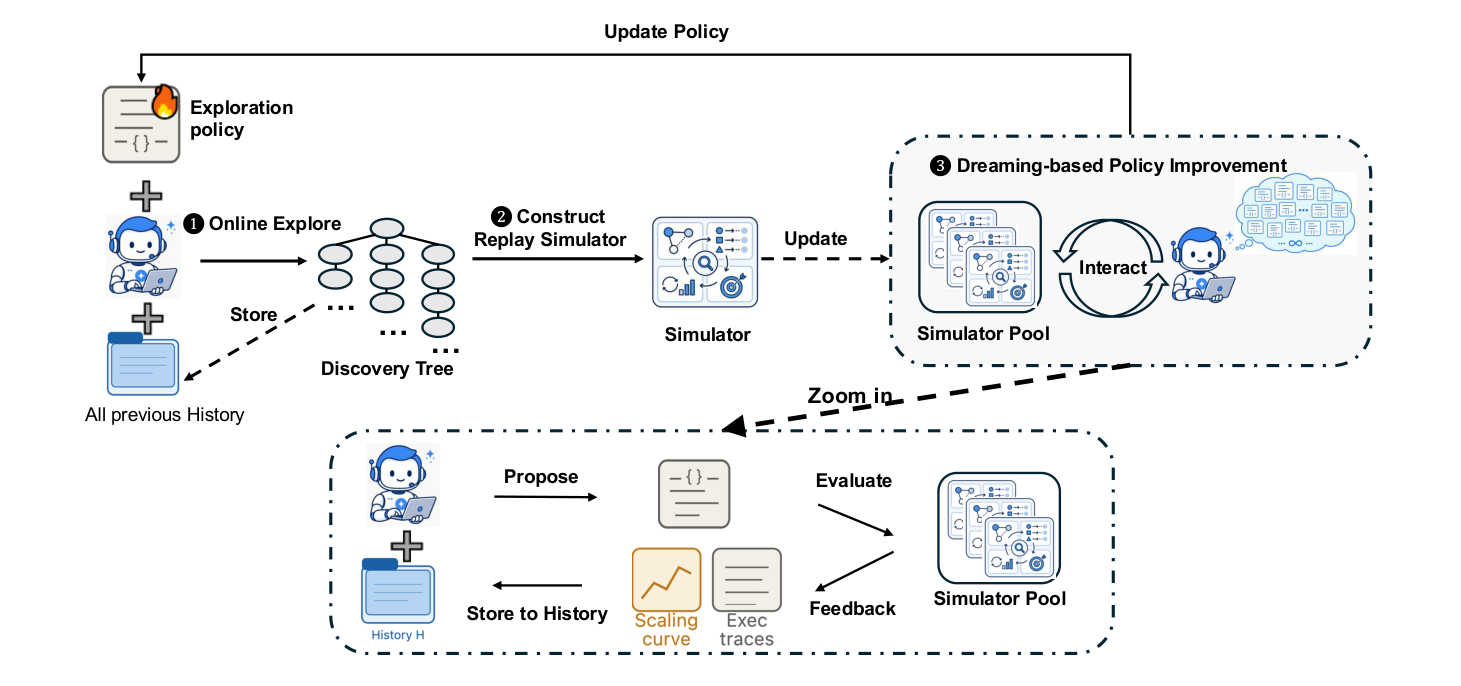
The system alternates between “online exploring” and “offline dreaming” across three stages:
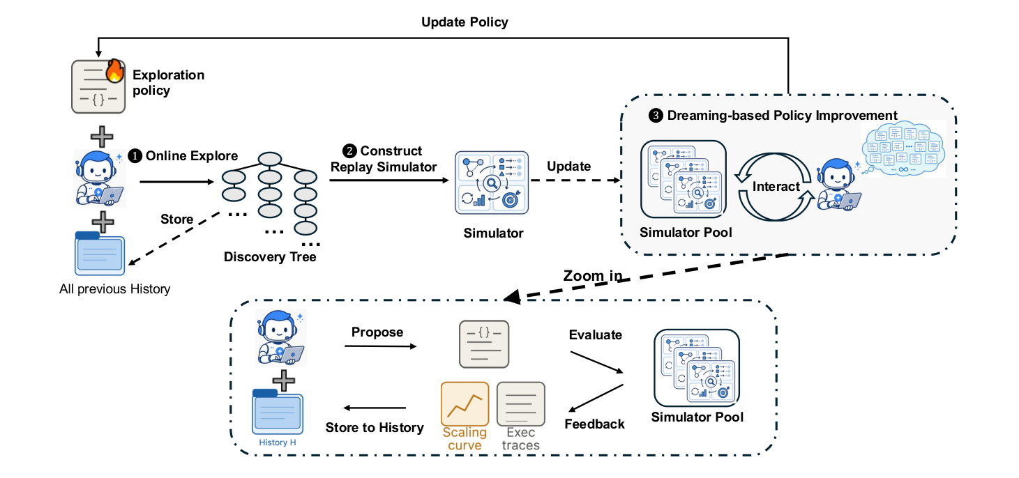
Stage one (Online Explore) uses the current exploration policy to direct a coding agent through a real discovery loop, logging every attempt as a discovery tree. Stage two (Construct Replay Simulator) folds that tree into a growing history pool. Stage three (Dreaming-based Policy Improvement) imagines a large pool of candidate policies against the history pool, replays each candidate against the stored trees to compute a score, and picks the best-performing version to become the policy that actually gets deployed next round. Once the loop finishes, it returns to stage one and starts a new round with the improved policy.
Notably, only the exploration policy’s code changes — the coding agent that actually solves problems, the evaluator that scores them, and the execution interface are all frozen. This “freeze most of the system, let only one small, controllable part self-improve” design is worth noticing as a pattern for dissecting self-improving systems in general, independent of this specific paper.
3.1 The discovery tree: history you can replay but never rewrite
Every node in the discovery tree represents one “generate-and-evaluate” attempt. The paper formalizes it with a small set of symbols:
- : the root node, representing the initial workspace state.
- : a non-root node in the tree, representing one attempt.
- : ’s parent node (can be , or another ) — when the agent produces , it continues from ’s saved workspace, using its accumulated observations as context.
- : the score of attempt (higher is better).
A node stores more than just a score — it includes a filesystem snapshot, the produced artifact, and evaluation diagnostics, making it a complete, replayable record of that attempt. At any point, only two kinds of nodes can be extended further: the root node (opening an entirely new branch), or an existing leaf node (continuing a branch already in progress). The paper writes this selectable set as , where denotes every leaf node currently in tree . Given parallel workers, the policy selects a batch of at most size from each round.
A small concrete example () is much easier to follow than the formula:
Round 0: T0={r}, A(T0)={r}, select C0={r}
         -> produces v1 (0.42), T1={r,v1}

Round 1: A(T1)={r,v1}, select C1={r,v1} (batch size=2, uses full W)
         -> r opens a new branch, produces v2 (0.55)
         -> v1 continues, produces v1a (0.51)
         T2={r,v1,v2,v1a}   (v1 is no longer a leaf)

Round 2: A(T2)={r,v2,v1a}
         select C2={v2,v1a}
         ...and so on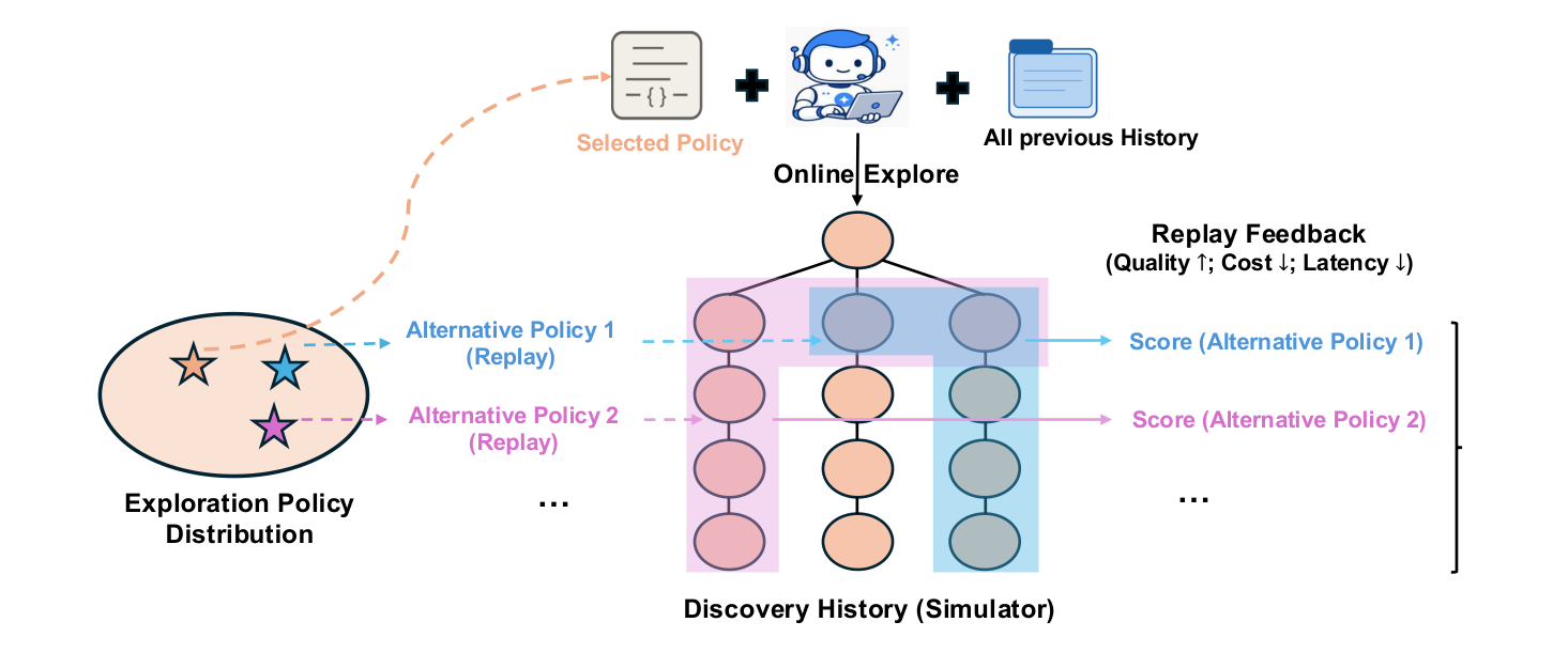
3.2 Online rollout and offline replay: same rules, two different logics
This is the fundamental mechanism behind everything the paper saves in cost. Online and offline use the same rules for “picking a node, forming a batch,” but the underlying logic is completely different:
| Online rollout (genuinely executing) | Offline replay (reading, not executing) | |
|---|---|---|
| Where node content comes from | The coding agent generates it live; the evaluator scores it live | Read directly from content already stored in the historical tree |
| Does the same action give a different result? | Yes (stochastic) | No (deterministic) |
| Which child does selecting root return? | Generates a brand-new branch live | Always the “earliest-created, not-yet-revealed” child in the historical tree — order entirely fixed |
| When selecting an already-expanded node | Generates a brand-new child live | Directly returns the child already stored in history |
Online rollout stores the newly built tree into the history pool at the end of every outer iteration; offline replay instead replays every tree accumulated so far, evaluating the same candidate policy version’s performance across all of history rather than just replaying the most recent one.
A full worked example is the clearest way to feel the difference. Suppose real online exploration left behind this complete historical tree ():
graph TD
    r["r
root node"]
    v1["v1
round 1 · 0.42"]
    v1a["v1a
round 2 · 0.51"]
    v1a1["v1a1
round 3 · 0.58"]
    v2["v2
round 2 · 0.55"]
    v2a["v2a
round 3 · 0.60"]
    r --> v1
    r --> v2
    v1 --> v1a
    v1a --> v1a1
    v2 --> v2a
The two branches were created in order — v1 before v2 — and replay locks that order in.
Replaying this tree with an alternative policy :
Round 1: select C={r} -> returns r's earliest-created, unrevealed
         child = v1 (0.42)

Round 2: A={r,v1}, select C={r,v1}
         -> r: returns the next unrevealed child = v2 (0.55)
         -> v1: returns its only child = v1a (0.51)

Round 3: A={r,v2,v1a}, r has no children left to reveal,
         select C={v2,v1a}
         -> v2: returns v2a (0.60)
         -> v1a: returns v1a1 (0.58)
         everything revealed -> stop
It takes only 3 rounds to reveal the entire tree, and every round fills the full — if the original online exploration expanded branch by branch, round by round, without ever fully using its parallelism, this alternative policy’s replay result reveals exactly that: it should have batched more aggressively from the start. That’s exactly where replay’s value lies: you don’t have to re-execute any code at all, you just read the existing record in a different order or grouping and can already see the efficiency difference between policies.
3.3 Avoiding “the winner is always whoever traverses the whole tree”
Looking at the highest score revealed during replay isn’t enough on its own — traversing the entire tree always yields that tree’s global best score, which fails to distinguish “efficiently finding a good result” from “brute-forcing the whole thing.” The paper’s replay score is therefore made up of three terms: the highest score among revealed nodes (quality), minus the number of revealed nodes times a coefficient (cost — the more you reveal, the more you’re penalized), plus the average number of revealed nodes per round times another coefficient (a parallelism bonus, rewarding policies that know how to batch). The main text denotes these two coefficient weights and , but never states the actual values used in the experiments, either in the main text or the appendix.
A concrete example makes the design’s intent clearest. Using the same tree as before, suppose and (illustrative values, not the paper’s actual settings):
| Nodes revealed | Highest score (quality) | Nodes revealed | Avg. revealed/round (parallelism) | Formula | Score | |
|---|---|---|---|---|---|---|
| Policy A (conservative, sequential) | v1, v1a, v1a1 | 0.58 | 3 (1 per round, ) | 0.53 | ||
| Policy B (aggressive, batched) | all 5 | 0.60 | 5 (2 each in rounds 2, 3, ) | 0.5167 |
Policy B has both a higher top score and higher parallelism, but because it revealed two more nodes, the cost term deducts more, and the final computed score actually favors the conservative Policy A — “conservative but precise” beats “aggressive but wasteful.” That is the core intent of this scoring formula: it’s not simply about who scores highest, but a trade-off between “how good” and “how expensive,” with the balance entirely determined by and . Also, a candidate policy’s final score is the average of scores computed separately across all historical trees:
not a score from a single tree — otherwise the chosen policy might just happen to fit that one tree’s particular structure and fail on a different one.
3.4 A “never gets worse” safety net
Each round of policy improvement works like this: first, let the currently deployed policy replay itself, unchanged, to get a baseline score . Then a policy-development agent (itself an LLM), whose job is to rewrite code, reads this replay record and produces a new version , which also gets replayed and scored. This process repeats up to , producing versions in total. Finally, among all candidate versions, the one with the highest replay score () is picked to become the policy that actually gets deployed next round.
The candidate pool always keeps the “completely unchanged” original version , so the picked score is never worse than the original — worst case, none of the rewrites improved anything, and you just keep using the original instead of regressing from a bad edit. This design is called monotonic non-regression, and it’s a simple health-check that any “LLM edits its own logic” system can be checked against: does the candidate set always keep an “unchanged” option as a floor?
There are actually three roles in the full pipeline that potentially involve an LLM, and knowing which is expensive and which is cheap matters — including whether the evaluator itself is LLM-based at all, which the paper never states:
| Role | Which prompt | What it produces | When it runs | Cost |
|---|---|---|---|---|
| Discovery agent | Appendix B.1 | The candidate solution content for the task | Only during Online Explore | Expensive (actually solving the problem) |
| Evaluator | Not stated whether it’s an LLM | Score | Only during Online Explore | Usually cheap (running code to measure) |
| Policy-development agent | Appendix B.2 | The exploration policy’s code | Dreaming stage, runs times per round | Moderate (rewriting code, no need to actually solve the task) |
| Replay itself | No prompt, pure program logic | Score | Dreaming stage, runs for every candidate version | Nearly free (pure table lookup) |
Genuinely expensive LLM calls only happen in role 1 (a limited number of times) and role 3 ( times per round, usually single- to double-digit) — replay scoring itself involves no LLM at all. That’s why “thousands of candidate policy evaluations” doesn’t turn into thousands of expensive API calls.
That said, this safety net has an easily overlooked limitation: it guarantees only that “the replay score doesn’t regress,” not that “real online performance doesn’t regress” either. That gap is the replay-to-real gap, and it’s unpacked fully later.
3.5 The engineering details buried in the appendix: how the B.2 prompt is designed
The paper’s appendix includes an approximately 270-line prompt that guides how the policy-development agent rewrites the exploration policy’s code. This prompt is the highest-value piece of engineering in the entire paper, and a few of its core mechanisms are worth pulling apart:
The prefix-only constraint: every decision the policy makes may only use “nodes this particular replay has itself actively revealed so far” — never the score of an unrevealed node, budget statistics, or any “god’s-eye-view” information. This prevents cheating — scanning the whole tree upfront for the highest score and pretending exploration happened to find it — because real online deployment offers no such opportunity to cheat, since the online tree hasn’t even grown yet. This restriction — decisions can only use what’s currently known, never peek at the future or the global picture — is a standard requirement in reinforcement learning and online algorithms called the causality constraint. It isn’t something Dream-RSI invented (off-policy evaluation follows the same logic).
A three-way split for batch decisions: each round selects up to candidate nodes to form a batch, and the prompt requires composing it from three roles — exploitation (extending the currently most promising line normally), exploration (opening a new root, or digging deeper into an under-explored branch), and recovery (at most one, a genuinely repairable failed attempt). This is fundamentally the classic multi-armed bandit explore-exploit trade-off, but with an added recovery role that isn’t part of the traditional bandit framework, because “failure” here might just be an implementation bug rather than the direction itself being bad. The rules explicitly require: recovery takes at most one slot and can never crowd out exploitation’s slot or leave a worker idle; it can’t use a fixed quota — it has to be decided dynamically based on prefix evidence; and random sampling, or picking a candidate “just because it’s obviously good,” are both prohibited.
A four-way failure taxonomy: hard-unrecoverable (definitely can’t be fixed), repairable implementation failure (the idea might be fine, it’s an implementation bug), weak-but-underexplored (mediocre score but not yet tried deeply enough), and repeatedly unpromising (there’s already enough evidence this direction genuinely doesn’t work). One easily overlooked detail: valid==False doesn’t mean “failure” — an attempt’s code might run to completion without throwing an error, yet the produced solution still fails to satisfy correctness conditions; that’s a normal evaluation that produced a weaker solution, not something that should be dumped into the “repairable failure” bucket and retried. And no classification is ever a permanent verdict — even if a branch is judged hard-unrecoverable, a single subsequent successful result reopens that branch. The bigger context behind this framework — including its relationship to classic distributed-systems design and how it maps onto an agent’s tool-calling error handling — gets fully unpacked later in the “Failure Classification” section.
Beta: the policy’s internal conservative/aggressive dial: beta in the prompt is a hyperparameter internal to the policy’s own code that determines how lenient or conservative its behavior is — it is not the same thing as / from the main-text formula. The main text uses /, while the appendix’s implementation uses beta alongside a different set of symbols (pareto.reward, pareto.auc, lambda), and the paper never clarifies how the two correspond.
Grid planning: before a brand-new round of online exploration begins, there’s an even earlier decision — how many root branches to open (width), and how many levels deep to extend each one (depth). This is handled by a separate plan_grid() method, which likewise cannot peek at this round’s not-yet-happened results and can only decide based on the history of past rounds. The rough decision rules: if many directions show early promise but stall once explored deeper, increase width; if high scores only emerge after refining many levels and are concentrated in few directions, increase depth; if directions are already explored deep enough but still stalled while untried types of directions remain, increase width; if failures repeat as hard failures or directions are highly redundant, scale both width and depth back conservatively.
A concrete illustration makes this easier to picture: if only one root branch kept producing high scores through refinement over the past three rounds while every other branch stalled at depth two, plan_grid() should conclude “the direction is already found — worth digging deeper,” and increase depth next round rather than opening more width. Conversely, if every branch stalls around depth 4-5 with no further progress but several entirely untried starting approaches remain, the conclusion should instead be “open a few new roots and look for a better starting point,” rather than keep forcing progress on a direction that’s already stuck.
Dream-RSI’s adaptive mechanism is therefore layered: the outermost layer is the grid (arena size), the middle layer is beta (conservative vs. aggressive play style), and the innermost layer is the round-by-round concrete decision logic (prefix-only, batch portfolio, failure classification). This “layer the adjustable knobs by timescale” architectural approach is, even independently of this specific paper, a pattern worth referencing when designing any system meant to self-adjust across iterations.
4 Three experimental domains: what’s saved is compute, not quality
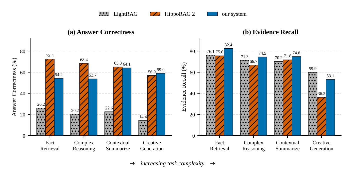
The paper tests Dream-RSI across three domains: algorithm engineering (using the Lasso regularization path as an example), mathematical optimization (Sum-Difference, Autocorrelation, and Circle Packing), and GPU kernel engineering (four tasks from KernelBench). There’s a common pattern across all three worth stating up front: nearly every dimension Dream-RSI wins on is “reaching the same quality with less compute,” not “quality itself breaking new ground.”
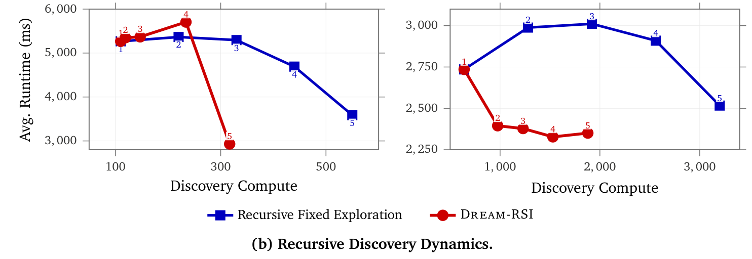
In algorithm engineering, Dream-RSI matches or beats the baseline’s wall-clock runtime on six held-out downstream tasks, while using one to two orders of magnitude fewer discovery-agent calls:
Mathematical optimization is the domain where “almost no quality improvement” is most obvious:
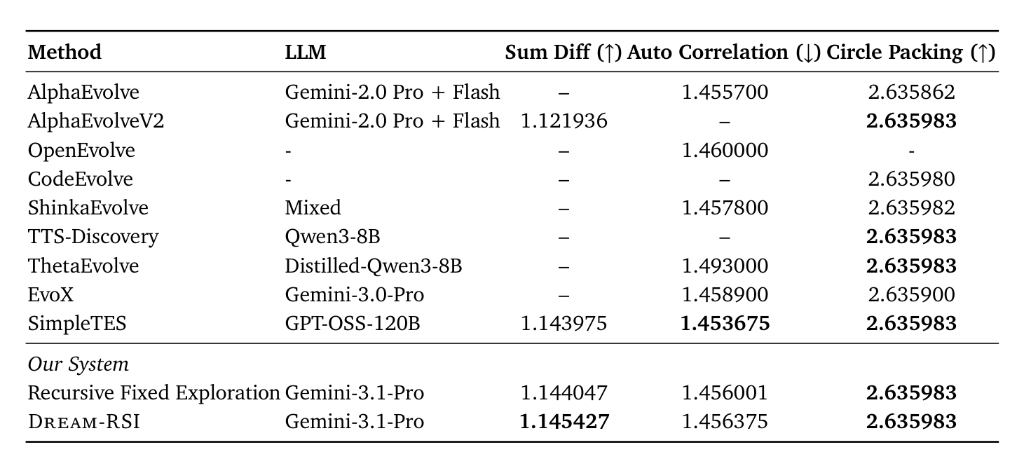
Dream-RSI reaches comparable scores with far fewer generations than SimpleTES (the other baseline system used as a control for these three math tasks) — under 1,000, versus SimpleTES’s 51,200 — but the actual score gaps mostly sit three or four decimal places out, and on Circle Packing every method converges to the same value.
GPU kernel engineering is where the efficiency gain reads most directly:
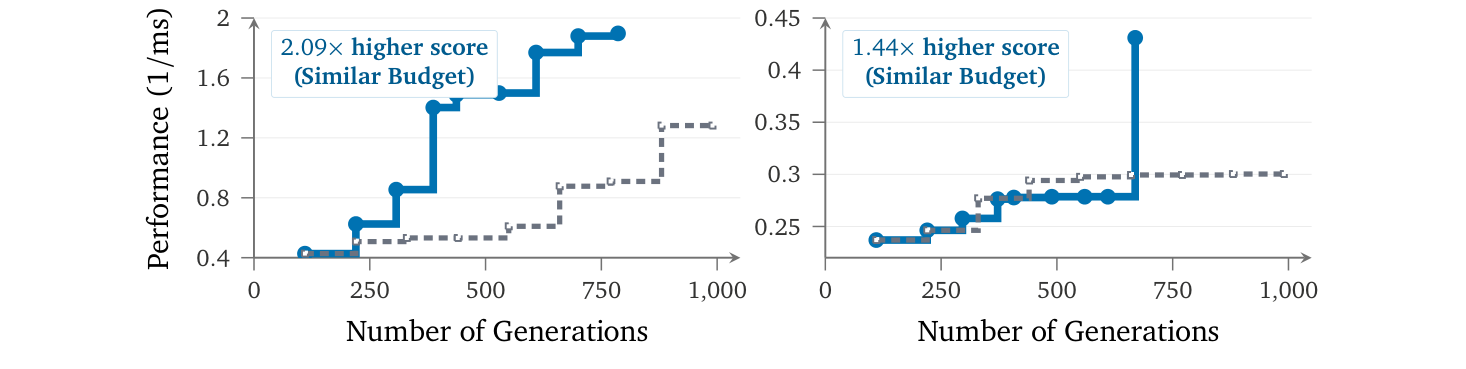
Looking at all three domains together, there’s a shared blind spot buried in the paper’s own efficiency metric, and it happens to be a domain with concrete numbers that lets you estimate the scale of it: on the Lasso task, Gemini-3.7-Flash’s online exploration used 32 parallel workspaces per round, each running up to 20 refinement steps, accumulating 1,879 discovery-agent calls across five rounds — and by the start of round five, the previous four rounds had already left thousands of records to read. As the number of rounds grows, in principle the context each API call needs to read only gets longer and more expensive, but the paper’s efficiency metric throughout only counts “number of discovery-agent calls” and never accounts for this. This issue applies to all three domains; Lasso simply happens to be the only place the paper reports concrete call counts. This gets pulled out and unpacked on its own in the “Will accumulated history blow out the context?” section below, including where it might hit a ceiling and more general fixes.
5 The ablation and how exploration behavior evolves
More than the three main experiments, the ablation in §5.1 is worth a closer look, and is in some sense the most methodologically valuable part of the whole paper: it compares “treating history as an interactive replay simulator to actively test against” versus “summarizing history into a text prompt to guide direction.” Both paradigms tested (Dream-RSI and another baseline) got worse once the text-prompt guidance was added.
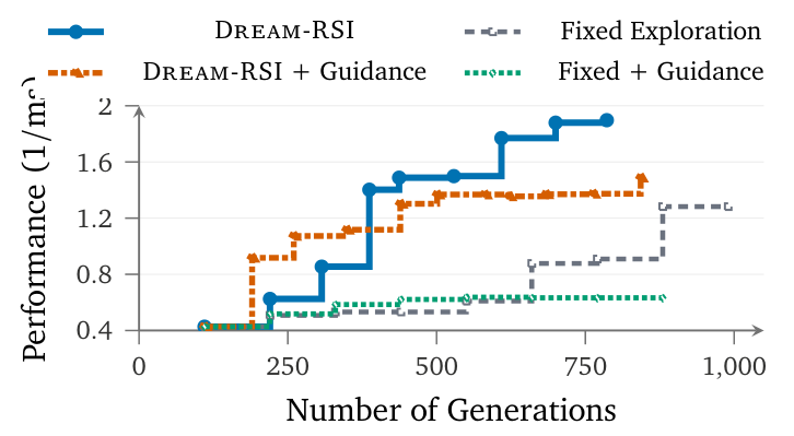
The paper’s interpretation is that in long-horizon, multi-threaded exploration, hard-coding directional suggestions into the prompt actually over-constrains the search space and suppresses exploration diversity. This result is worth placing in a broader context: on the same underlying problem — how to make use of past experience — approaches like ReasoningBank and WikiSkill take the route of “summarize experience into text knowledge and inject it back in.” This ablation points toward “structured, executable replay” outperforming “text-summary-style prompting” in the specific context of exploration policies — but that’s a result from one setting, and it doesn’t generalize into a claim that summary-based memory methods are broadly inferior to structured replay.
Another experiment tracks how the learned exploration policy’s own behavior changes as recursive rounds accumulate.
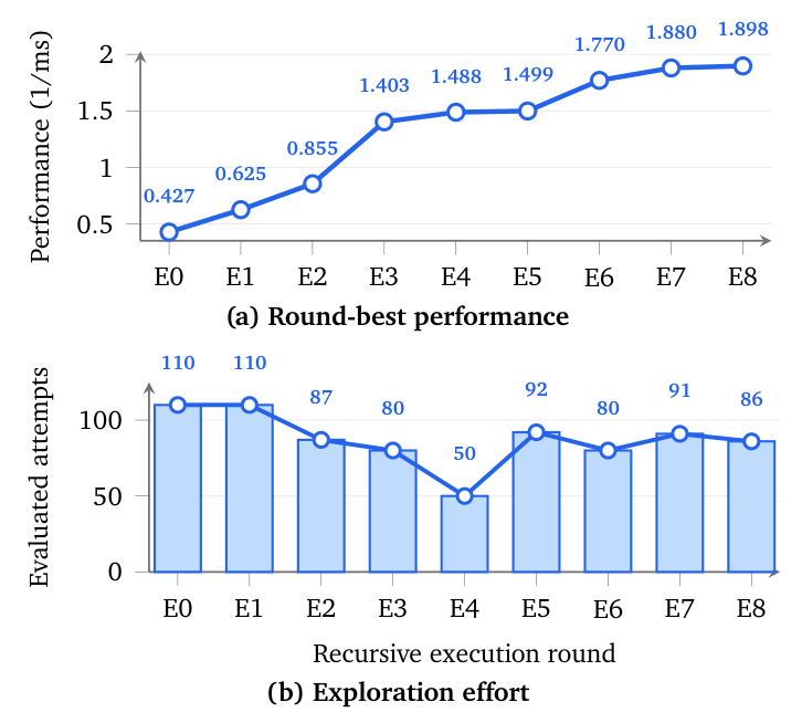
The paper observes a clear adaptive pattern: early on, while performance is still improving quickly, the policy tends to be conservative, spending resources digging deeper into a few promising-looking branches. As performance approaches a plateau and progress slows, the policy shifts toward more aggressively opening new branches and widening the search. This “early convergence, late divergence” behavior isn’t a hard-coded rule — it’s something the policy learns on its own from historical replay, echoing, to some degree, the plan_grid() logic discussed earlier that dynamically adjusts exploration width and depth based on history.
6 How much does this paper honestly accomplish?
Laying the method and experiments out flat, Dream-RSI’s core contribution is real: reframing “a completed exploration history” as a data structure that supports off-policy evaluation, used to cheaply screen improved versions of an exploration policy instead of expensive online trial and error — and the ablation genuinely confirms it beats simply summarizing history into a text prompt.
But honestly, the contribution doesn’t carry much weight. Quality improvement is almost nonexistent — most gaps on the math-optimization tasks sit three or four decimal places out, and Circle Packing is a dead tie — the real contribution clusters around “reaching the same quality with less compute,” an efficiency contribution, not a capability breakthrough. The “World Model” framing has a substantive gap from an actual world model, and its more accurate positioning is a sophisticated off-policy replay evaluation mechanism — a point worth unpacking fully, and the part this post spends the most space on from here.
7 Beyond the paper: a few transferable design habits
What follows relates to Dream-RSI less as “the subject of this post” and more as “the paper that happens to be the trigger.” Even if you’d never heard of Dream-RSI, these things hold up on their own, and there’s a good chance they’ll come in handy the next time you design an agent system — this is the part of the post that gets the most space from here on.
7.1 Is this really a “World Model”?
Dream-RSI frames the whole mechanism as analogous to a “World Model,” echoing Dreamer-style model-based RL systems. That analogy sounds impressive, but it doesn’t hold up under close inspection.
RL basics first: the basic reinforcement learning loop is “agent observes a state → picks an action → environment gives feedback (reward + new state) → loop.” The goal is to learn a policy: given a state, what action to take to maximize long-run cumulative reward. Two branches split off from here.
Model-free: the agent learns entirely through actual interaction and trial-and-error with the environment, slowly learning “is taking this action in this state good in the long run,” without ever learning “how the environment itself works.” An analogy: learning to ride a bike relies on muscle memory, not an understanding of Newtonian mechanics.
Model-based — where the world model comes in: the agent additionally learns an “environment dynamics model”: input “current state plus action,” output “next state plus reward.” This model is the world model. With it, instead of actually interacting with the environment, the agent can just keep asking the model “what happens next if I do this,” and simulate entirely inside the model. An analogy: a chess grandmaster mentally rolling out the next five moves relies on an internal model of how the rules of chess work. Real-environment interaction is often slow, expensive, and risky; with a sufficiently accurate world model, the agent can “practice” cheaply and at scale using standard RL methods inside the model, since each step is just one forward pass of the model rather than actually executing an action — this is the fundamental reason model-based RL is usually more sample-efficient than model-free.
But there’s a crucial precondition here: for a world model to be useful, it must be able to generalize to “state-action combinations that have never actually been visited” — otherwise it can only replay things that have already happened, which would be pointless.
Concretely, this is how Dreamer does it: it first compresses high-dimensional input (game frames) into a low-dimensional latent vector z (the latent state), rather than predicting directly in pixel space. It then learns a function inside this compressed space — “current z plus action a → predicted next z’ plus reward” — and this function (often called an RSSM, Recurrent State-Space Model) is the core of the world model, trained on data collected from real interaction. The “dreaming” process then unfolds entirely inside latent space: starting from some z, repeatedly “use the policy to decide action a → use the dynamics model to predict z’ → decide the next action,” rolling out an entire imagined future trajectory — never touching the real environment, and never decoding back to real frames. The full loop looks like:
graph TD
    A["Real environment interaction"] --> B["Collect frame, action, reward data"]
    B --> C["Train encoder + dynamics model
(world model)"]
    C --> D["Imagine many future trajectories
in latent space (dreaming)"]
    D --> E["Train / improve the policy
on imagined trajectories"]
    E --> F["Deploy the improved policy
to the real environment"]
    F --> A
The dynamics model is a neural network, which is fundamentally a learned continuous function — it usually produces a reasonable prediction for z-and-a combinations that are “similar to, but not identical to” anything it has seen before. That’s exactly where its ability to generalize to unseen states comes from.
This is exactly the gap between Dream-RSI and a genuine world model. Dream-RSI’s “replay simulator” doesn’t have this ability: discovery tree replay stores nodes that have already happened, verbatim, and replays them — there’s no function doing generalization or interpolation anywhere. If a branch was never explored, replay is simply empty for it and produces no prediction to evaluate. Calling Dream-RSI’s mechanism a “World Model” is, to some degree, overselling it; a more accurate positioning is a sophisticated off-policy replay evaluation mechanism.
7.2 Why not just search with a world model at every single step?
A natural question: if you already have a world model that generalizes, why not just try every action at every state and pick the one with the highest reward, at every step — wouldn’t that find the reward-maximizing trajectory directly?
This approach genuinely exists — it’s called Planning, with concrete techniques like MPC (Model Predictive Control) or CEM (Cross-Entropy Method): at every timestep, use the world model to forward-simulate several candidate action sequences, pick the one with the highest cumulative reward, execute its first step, and re-search from scratch at the next timestep. Dreamer’s predecessor, the PlaNet paper, did exactly this — planning directly in latent space with CEM, without learning a separate policy at all. Dreamer later switched to learning a policy instead, for specific reasons — and those three reasons are themselves worth remembering:
Problem one: in a continuous action space, there’s no such thing as “having tried every action.” In the scenarios Dreamer targets (robot control, continuous Atari-style operation), actions are often continuous-valued, so you can sample at most a few dozen or few hundred candidates — this is no longer “finding the optimal solution,” it’s “approximating by sampling.”
Problem two: search compute explodes exponentially with horizon. Suppose you try 10 discretized actions per step and plan 15 steps ahead: that’s combinations — and this is the amount of compute needed to be recomputed at every single real timestep, which is completely infeasible for anything requiring real-time response. MCTS uses heuristics to prune away most meaningless branches, but even with pruning, the compute cost is still far higher than “train a policy network once, and at decision time just do a single forward pass.”
Problem three: planning far into the future accumulates and amplifies the model’s prediction error. Planning 15 steps ahead means feeding “a step-1 prediction that already has error” into the model to compute step 2, then feeding an even-more-erroneous result into step 3, and so on — the error compounds as you go, so searching deeper actually increases the risk of being misled by an increasingly inaccurate model.
Dreamer’s solution is to move the search cost into the training phase: train a policy plus a value function, both trained on a large volume of imagined trajectories. The imagined trajectories used during training don’t need to be long, because the value function itself absorbs the job of estimating “roughly how much value the rest of this path holds” (a bootstrapping trick — you don’t have to actually simulate all the way to the end to know if a path is good). Once trained, real deployment-time decisions are just a single forward pass of the current z through the policy network — no need to re-search at every timestep in the real world. The search cost gets moved to background training, and real-time decisions become cheap.
Comparing all three approaches side by side makes this clearer:
| Approach | How it picks an action at decision time | Pros | Cons | Representative methods |
|---|---|---|---|---|
| Planning | Re-search/re-simulate with the model at every step | No separate policy to learn; more “honestly” uses the model | Can’t search continuous action spaces effectively; expensive at decision time; error accumulates over long horizons | PlaNet, MPC, CEM |
| Policy Learning in Imagination | A single policy forward pass at decision time | Cheap at decision time; the value function handles long-term return via bootstrapping | Policy quality is capped by how accurate the world model is; requires an extra network to train | Dreamer (v1-v4) |
| Hybrid | Use policy/value as a prior to narrow the search, then do a shallower search | Combines both sides’ advantages; guided search avoids flailing | Highest system complexity | MuZero, AlphaZero |
The transferable rule: when the action space is small and discrete, a single-step model computes quickly, and you can tolerate spending more compute at decision time (turn-based board games) — lean toward pure planning or a hybrid approach; when the action space is continuous, real-time response is required, and the horizon is long — lean toward Dreamer’s approach of moving the search cost into training. This “move the expensive computation to the background so real-time decisions stay cheap” idea is a general system-design principle, not specific to RL — MemRL’s move of treating memory retrieval itself as a policy trained via RL, rather than re-judged live every time, is another application of exactly the same cost-shifting logic.
7.3 Will accumulated history blow out the context?
As mentioned earlier, the exploration prompt in the appendix explicitly requires the agent, before proposing a new plan, to read through every sibling attempt’s proposal and every record in the complete history — explicitly not sampled, not just the most recent rounds, not just the current branch. Pulled out and examined on its own, this is a gap the paper never addresses at all, and it isn’t unique to Dream-RSI — any long-running agent system has to deal with it.
The problem is that history is cumulative — by the start of round five, the previous four rounds have already accumulated every generated node, potentially thousands of proposals. If every new attempt has to read through all of that content before it can begin, then the context length of every API call grows linearly with the round count — or even faster, since sibling nodes within the same round also have to read each other — and the cost and latency of every call keeps growing the further the rounds go. But the paper’s efficiency metric throughout only uses “number of discovery-agent calls” as cost, never accounting for “each call itself getting more expensive as context grows longer,” and nowhere in the paper is there any mechanism for context management, summarization, retrieval-based reading, or a reading cap.
The more general question is: should an agent stuff its entire history into context, or instead use a retrieval-based (pick only what’s relevant), summarization-based (compress before inserting), or hierarchical (wiki-style, tiered management) memory mechanism — this is a design choice any long-running agent system has to face. The paper itself cites approaches like ReasoningBank in its Related Work section, yet never applies the same concern to the history-reading design of its own exploration prompt — an inconsistency worth noting.
7.4 What is replay actually replaying?
An easy point of confusion: “at a given node, the policy can’t take a different action” — this intuition is correct, but you need to be precise about what “action” actually refers to here.
“Action” does not mean “deciding what content to generate at node ” — that part is frozen; ’s children’s content was already generated and stored in the tree back when real online exploration happened, and replay never regenerates it. The real “action,” at every round’s decision point, is which nodes the policy selects from to put into batch — who to pick, how many together, in what order, and when to select an empty batch and stop. That is the one and only thing that varies, and the one thing that’s genuinely different between policies. Put plainly: the tree’s “content” is dead (whose child is whose, what score, all fixed), but “how you plan to walk this tree” is alive — that’s what the policy is actually doing.
There are two easily confused pieces of code here, and it’s worth keeping them straight:
| What it is | Who produces it | Which prompt guides it | Scope | |
|---|---|---|---|---|
| Exploration policy | Code that decides how to walk the discovery tree | The policy-development agent (LLM) | The B.2 replay-improvement prompt | RSI-loop level — manages whether to open new branches, batch size, when to stop |
| Task solution (e.g. the Lasso solver in the paper’s Appendix C) | The actual candidate-solution content inside one specific discovery-tree node | The discovery agent (the coding agent that actually solves the problem) | The B.1 exploration prompt | Single-node level — what a given attempt concretely produced |
The Lasso solver code shown in Appendix C is the content of the highest-scoring node in the discovery tree after Dream-RSI finishes running — it has nothing to do with the “exploration policy” at all. It’s the answer to the task itself, not the logic for “how to walk the tree.”
Back to the Policy A / B example from earlier: neither policy, at any step, regenerates any content — the v2, v1a, v2a, and v1a1 nodes Policy B reveals would be identical to what Policy A would reveal if it happened to select the same nodes, because both are reading the same stored record. The only difference is at the decision level: who to select, in what order, with what batch size, and when to stop. The payoff of this is direct: if A and B each ran a real online exploration in the real world, that would cost two genuinely expensive rounds of coding-agent generation plus evaluator scoring — potentially hundreds of API calls and actual code execution. But comparing how efficiently A and B “walk” the same already-existing tree, two replays together might take milliseconds, since it’s just reading a tree structure sitting in memory. That lets you cheaply test thousands of walking strategies, screen for the most efficient one, and only actually deploy the single one you finally chose online.
7.5 The replay-to-real gap: two independent sources
As noted earlier, monotonic non-regression only guarantees “the replay score doesn’t regress” — it says nothing about whether “real online performance doesn’t regress” either. This gap has two independent sources, not a causal chain — they’re easy to lump together as one thing, but pulling them apart is more precise.
Source one: the beta (/) setting might not reflect what you actually care about. Even if replay could see every possible path in the universe, if is set too high (over-penalizing cost), the selected policy would still get pushed toward “reveal as little as possible,” even when that’s a suboptimal choice in the real world. This gap comes from whether “what this scoring formula measures” actually equals “what we care about” — it has nothing to do with how much of history the tree covers.
Source two: a replay context is, after all, a historical context, not a real environment. Even with perfectly tuned , replay can still only choose among branches that have already been walked, and cannot evaluate any possibility that was never explored. This gap does not go away, because it has nothing to do with whether beta is well-tuned — it comes purely from “how big this simulator’s world is.”
Verifying these two sources are genuinely independent doesn’t take much — a simple thought experiment suffices: suppose beta is tuned perfectly but the tree is still just a historical tree — the gap still exists (from source two). Conversely, suppose the tree covers every possible branch (idealized) but beta is poorly tuned — the gap still exists (from source one). In both hypothetical scenarios, removing one variable doesn’t make the other gap disappear, which proves the two exist in parallel, independent of each other.
The paper treats the two very differently. For “beta isn’t set right,” the paper does attempt a fix — the appendix designs a beta sweep plus an adaptive default-beta rule that recalibrates next round’s default based on the previous round’s real online performance, which is, in a sense, using real feedback to correct the objective function itself. For “replay can only see history,” the paper has no particular remedy — the only way to shrink this gap is the overall RSI loop itself: every online exploration round adds another tree to the history pool, so the world the simulator can replay keeps growing. But that only expands the “known world” after the fact — it doesn’t solve the in-the-moment limitation that, at the point of any given round’s decision, the simulator simply cannot see possibilities that haven’t happened yet.
This breakdown is itself a transferable framework for judgment: any system that uses historical data for off-policy evaluation can ask itself these two questions — does what the scoring formula measures actually equal what I care about? Does the range covered by historical data actually approximate the real situation I need to decide in? The answers to the two questions point to different remedies — they can’t be conflated and solved with a single approach.
7.6 Failure classification: from distributed systems to agent tool-calling
The paper’s appendix requires the policy-development agent to write failure-classification logic into the exploration policy’s code — the four categories were already listed earlier (hard-unrecoverable, repairable implementation failure, weak-but-underexplored, repeatedly unpromising). What’s worth doing here is placing this framework into a bigger context, because it actually stands on the logic of two different fields.
Which errors are “usually” considered repairable: output/correctness mismatches, shared-memory/resource limits, variable/code errors, and mask/layout/shape errors. The appendix explicitly warns: seeing a generic error label like “compile_other” is not grounds to permanently declare the direction unrecoverable — it’s just a one-off compilation-issue label, not evidence the direction itself is flawed.
7.6.1 The bigger context behind this framework: transient vs. permanent
This problem was first, and most systematically, discussed in the field of distributed systems and cloud services — that’s this vocabulary’s native domain, not a general-purpose AI term.
Transient failure:
  - a network connection briefly drops, the server is momentarily
    overloaded, a request times out
  - characteristic: "just try again" is quite likely to succeed;
    the error has nothing to do with whether the request itself
    is valid
  - examples: HTTP 503 (server busy), lost network packets

Permanent failure:
  - the request itself is wrong: bad format, insufficient
    permissions, the resource genuinely doesn't exist
  - characteristic: "try 100 more times" gives the same result
    every time; the problem isn't luck, it's the content of the
    request itself
  - examples: HTTP 404 (resource not found), HTTP 401 (unauthorized)
In practice, the most common way to judge this is by HTTP status code family: 5xx (server-side problems) is usually treated as transient and worth retrying; 4xx (problems with the client request itself) is usually treated as permanent, where retrying is pointless. The accompanying retry techniques are old friends too: exponential backoff — wait 1 second before the first retry, 2 seconds before the second, 4 before the third, so you don’t hammer a server that’s already overloaded and make the overload worse; jitter — add a bit of random noise to the backoff wait time, so you don’t have 1,000 clients fail simultaneously and then retry at exactly the same moment, causing a new wave of collective overload (a problem with its own name — the thundering herd); and the circuit breaker — after enough consecutive failures against the same target, stop and pause for a while rather than keep trying, which maps directly onto Dream-RSI’s “repeatedly unpromising” category: once enough failure evidence has accumulated, stop wasting resources on that direction.
7.6.2 The third state that shows up in AI/agent settings
The traditional transient/permanent dichotomy assumes “retrying doesn’t accumulate new information just by trying more” — retrying a dropped connection 10 times doesn’t teach you anything more about the network link. But in a generative, exploratory setting like Dream-RSI’s, there’s a third state (this is an inference drawn from observation, not a term from the paper or an industry standard):
"Not enough evidence yet" (weak-but-underexplored):
  - not a "transient error" (nothing is broken, the score is
    just mediocre)
  - not a "permanent failure" either (no evidence this path
    doesn't work)
  - it's "too few samples so far to draw a conclusion"
  -> closer to "insufficient sample size for a hypothesis test"
     in statistics than to any "error type" in traditional
     retry logic
Dream-RSI’s design in this area is actually stacking the logic of two different fields on top of each other: whether the failure has a bug (the engineering/distributed-systems retry logic), plus whether this direction is worth continuing to invest in (closer to the evidence-accumulation logic of a scientific experiment). Organized into a transferable decision table:
| Situational feature | Category | How to handle it |
|---|---|---|
| The failure has to do with “this attempt’s luck”; retrying with unchanged content might still succeed | Transient | Retry directly, with exponential backoff |
| The failure is a problem with “the content of the request/direction” itself; retrying without changes gives the same result | Permanent | Don’t retry — abandon it or change the input |
| No failure, but the result isn’t good enough, and there have been very few attempts | Insufficient evidence | Don’t retry the same thing — explore a bit deeper via a different approach or angle |
| The same category of failure has already recurred many times | Circuit breaker territory | Pause investing further in this direction; move resources elsewhere |
The transferable rule: when designing any system that automatically decides whether to retry or keep investing, first ask whether this negative result relates to “the execution process” or to “the thing itself” (transient vs. permanent); if it’s a problem with “the thing itself,” ask whether the evidence on hand right now is actually sufficient to draw that conclusion (whether to first classify it as “insufficient evidence” rather than pronounce it dead on the spot). Asking these two questions separately, rather than relying on one blunt success/failure dichotomy, avoids two common mistakes: giving up too early on a promising direction, and stubbornly wasting resources on a direction that’s genuinely hopeless.
7.6.3 Applying this to an agent’s tool-calling error handling design
“Retrying” a tool call isn’t quite the same as “retrying” a network request — in traditional distributed systems, “retry” usually means “send the exact same request again,” but an agent’s tool call is generated by an LLM, which means there’s a richer spectrum of options beyond just “retry or not”: retry unchanged (only meaningful for genuinely transient errors), retry with corrected parameters (the tool itself is fine, the LLM just filled in the wrong parameters), switch to a different tool or approach (this direction itself might be wrong), or give up and escalate to the user (repeated failure, time to cut losses).
There’s a reasonably sensible way to split these four options between what the harness (program logic) handles directly and what should be handed off to the LLM’s judgment:
graph TD
    E["Tool call fails"] --> H{"Is the error structural?"}
    H -->|"Rate limit 429
503 / timeout"| A1["Harness auto-retries
+ exponential backoff
LLM never needs to know"]
    H -->|"Schema validation error
missing field, wrong type"| A2["Harness catches it before sending
asks LLM to regenerate parameters"]
    H -->|"Needs semantic understanding
can't be hard-coded"| L["Hand off to LLM judgment"]
    A1 -->|"retries exhausted"| L
    A2 --> L
    L --> L1["Parameter is semantically wrong
→ correct it and retry"]
    L --> L2["This tool keeps failing
→ switch tool or approach"]
    L --> L3["Several attempts, nothing useful
→ give up and ask the user"]
What the system prompt should provide is “judgment principles,” not an exhaustive error-code lookup table — real-world tool error messages are far too varied to enumerate. A more robust approach (borrowing from how the B.2 prompt itself is written — it gives judgment principles plus example characteristics, not a literal lookup table) is to put a principle like this in the system prompt: “if the error message indicates a parameter/format problem, try correcting the parameters and retrying once; if it still fails after two correction attempts, consider whether this tool is even applicable, or switch to another tool/report to the user” — while the harness ensures that whenever it does hand off to LLM judgment, it always includes the actual raw error message in context, rather than giving the LLM only an abstract “it failed” — only then does the LLM have something to actually reason about.
A concrete scenario makes this clearer. Suppose an agent calls an internal API to look up customer data, and gets back a 400 Bad Request with the message “invalid date format, expected YYYY-MM-DD.” The harness layer first judges: 400 isn’t a rate limit or timeout, so it’s outside the scope of automatic retry; the error message looks like a “parameter format problem,” not “the tool itself is unavailable”; so it passes this specific error message (along with “this is attempt number N”) back to the LLM. The LLM, given a judgment principle rather than a rule-by-rule list in its system prompt, reads “the date format is wrong,” classifies it as “repairable at the parameter level,” corrects the date format, and retries the call. If the same tool fails three times in a row (regardless of how many parameter corrections were attempted), a circuit-breaker-style principle kicks in: stop retrying indefinitely, and instead “confirm with the user” or “switch to a different data source.”
This design has a side benefit too: if every failed tool call gets tagged with a structured label (transient / repairable-with-correction / needs-different-approach / circuit-broken), those labels themselves later become great material for trace analysis — when reviewing a stretch of an agent’s execution log, you can quickly filter for “was this failure the tool being unstable” versus “was this the agent’s own judgment being wrong,” without having to eyeball the log line by line every time.
8 Conclusion
Dream-RSI’s core engineering insight is real: reframing a completed exploration history as a data structure that supports off-policy evaluation, used to cheaply screen improved versions of an exploration policy instead of expensive online trial and error — and the ablation genuinely confirms it beats simply summarizing history into a text prompt. But the contribution doesn’t carry the weight the paper’s framing suggests. Across all three experimental domains, the real gains almost entirely cluster around “reaching the same quality with less compute,” not a capability breakthrough — and the “World Model” framing has a substantive gap from an actual world model that can generalize to unseen states, so a more accurate description is a sophisticated off-policy replay evaluation mechanism.
Within the paper’s own method, there’s also one small thing worth remembering on its own: monotonic non-regression — the design pattern of always keeping an unchanged original version in the candidate pool as a floor — is a health-check any “LLM edits its own logic” system can be checked against.
But more than the paper’s own contribution, a handful of things this post’s second half pulled apart are worth remembering, and all of them stand independently of this specific paper: the habit of spotting a “fake world model” — whether it can evaluate possibilities that never happened is the first question for judging whether a “simulator/world model/imagination” claim is overselling itself; the cost-shifting logic between Planning and Policy Learning — moving expensive computation into training time; the fact that managing context for accumulated history is a design choice any long-running agent has to face, not a problem unique to Dream-RSI; the recognition that what replay actually replays is the decision logic of “how to walk the tree,” not the task content itself — a distinction that gives “offline-evaluating an online decision system using historical data” a clear boundary; the replay-to-real gap splitting into two genuinely independent sources that need to be diagnosed and remedied separately; and failure classification’s arc from the transient/permanent dichotomy of distributed systems, to the third “insufficient evidence” state that generative settings add, to how that framework maps directly onto an agent’s tool-calling error-handling design. These habits hold up independently of this specific paper, and are directly borrowable by anyone building a self-improving system or designing an agent’s error-handling logic.