EvoOntology: Self-Evolving Ontology for Data Agents

1 Data agents start from zero every time, and stuffing the prompt can make it worse
Ask a data agent (an AI agent that follows natural-language instructions to work on messy, mixed data: database tables, CSVs, documents, logs) a question like “Why did cost rise last month?” The answer may be scattered across several tables, or buried in a document. But the agent knows nothing in advance about what the data actually looks like: what the columns are called, how tables should be joined (linked through a shared column). So it has to feel its way through the data from scratch on every task.
EvoOntology: A Self-Evolving Ontology Layer for Data Agents (arXiv:2609.15779v1, from a team at Renmin University of China, 9/2026) takes this on by inserting a knowledge layer (an ontology) between the agent and the data. The agent can query it, and it patches itself based on how it gets used.
The core of that layer is an ontology. Think of it as structured domain knowledge: which business concepts exist, which database column each one maps to, which rules govern their use, all linked together as a graph. How this differs from a traditional ontology or a knowledge graph is covered in the extended reading at the end.
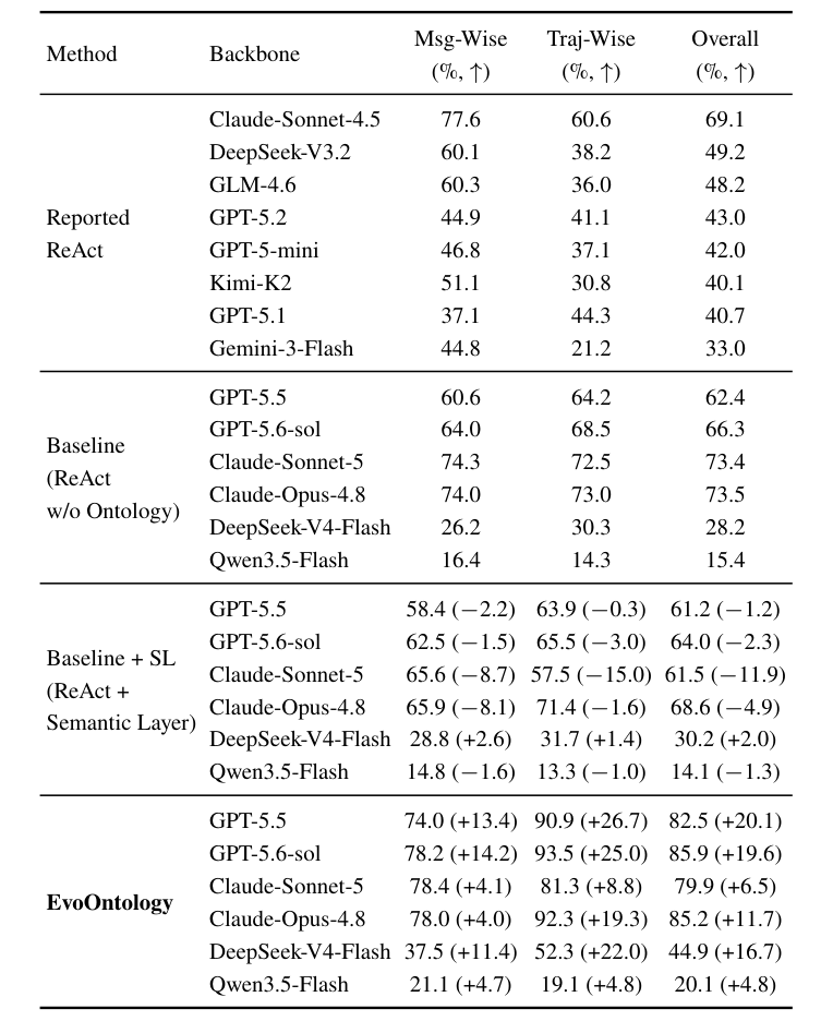
On DDR-Bench (an open-ended data-research benchmark; scores are accuracy, higher is better), EvoOntology beats the no-ontology Baseline across all six backbones (the underlying LLMs that drive the agent), gaining +17.8 points on average. The control that stuffs a semantic layer (a translation dictionary from business terms to database columns) into the prompt often does nothing or even loses ground: Claude-Sonnet-5’s Trajectory-Wise score (one of DDR-Bench’s metrics) fell by 15.0 points.
Still, the overall verdict is a modest contribution: its skeleton of a structured knowledge layer, attribution from failures, and a validation gate matches similar papers in spirit. What is worth borrowing is the design of the validation gate (a check a proposed change must pass before it is adopted), and the conclusion that actively querying beats stuffing everything into the prompt.
Some quoted blocks in the text begin with “The paper does not make this clear”. Those mark our own inferences or open questions after reading the paper, not the paper’s words.
The route: first the problem and the overall architecture, then how it cold-starts and how it evolves, then the experiments and our assessment, and finally a few ideas that hold up beyond this paper.
2 The problem: the agent does not know the data, and both existing approaches fall short
The core trouble: the agent reaches the data only through generic tools such as a SQL interface (the way you ask a database questions in a structured query language) or a file reader, yet it knows nothing in advance about how columns are named, how tables join, or what the contents look like. So every task starts with blind exploration: issuing probing queries over and over, guessing where the data might hide, then filtering the relevant bits out of a pile of irrelevant ones. The paper calls the gap between “what the agent knows” and “what the data actually looks like” the agent-data gap.
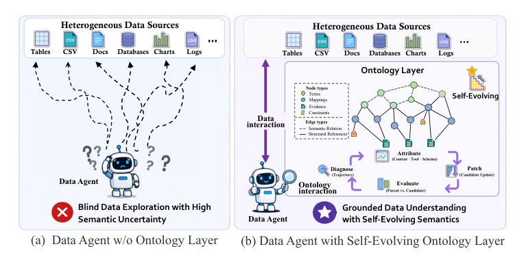
Figure 1 shows this in two panels. On the left, (a) is a data agent with no ontology layer: arrows point haphazardly at various data sources, labelled blind exploration under high semantic uncertainty. On the right, (b) adds an ontology layer in the middle, drawn as a small knowledge graph. The agent talks to this layer first, and the layer connects to the real data. It is labelled grounded data understanding, with semantics that evolve on their own.
So how do existing approaches deal with this gap? They fall into two camps:
| Approach | Examples | How it works | Limitation |
|---|---|---|---|
| Raw querying | Text-to-SQL agents such as DIN-SQL, MAC-SQL, CHESS | Let the agent poke at the schema (the structure of tables and columns) and issue exploratory queries | Once the data is large and heterogeneous, the agent falls into repeated, fruitless exploration; the column mappings it finally figured out this time must be rediscovered next task, so nothing it learns is kept |
| Semantic layer | dbt’s semantic layer, OWL ontologies | Humans pre-define which columns and metrics each business concept maps to, and the whole thing is stuffed into the prompt | A large data source exceeds the context-length limit; and the documents need manual upkeep, so every new data source or new task means more edits |
The semantic layer in that table is, intuitively, a translation dictionary between “business language” and “database language”. A user says “how much revenue last month”, but the database column may be called fact_rev.net_revenue_amt, and answering needs a join across three tables and the exclusion of cancelled orders. A semantic layer writes those translation rules down and sits between the data and the user.
Where OWL (Web Ontology Language) comes from: a W3C standard dating from around 2000, part of the Semantic Web and Knowledge Representation tradition, a completely different lineage from today’s LLMs and deep learning.
In today’s AI scene: not common. It lives mostly in traditional knowledge graphs, biomedical ontologies (Gene Ontology, for example) and enterprise data governance.
Its real strength is formal logical reasoning: once you define classes, subclasses and property restrictions, it can infer automatically. Define “all birds fly”, and when the system sees “X is a bird”, it concludes “X flies”.
Where the dbt semantic layer comes from: dbt (data build tool) is a popular data-engineering tool that handles SQL transformations inside a data warehouse. Its semantic layer feature (called MetricFlow underneath) lets a metric such as “revenue” be defined once, so every BI (business intelligence) reporting tool queries the same definition instead of each producing inconsistent results.
This is modern data-engineering practice, not an AI topic.
This paper’s angle is to upgrade the “static document stuffed into the prompt” into a layer that “the agent can actively query, and that evolves from usage experience”. The layer is wrapped as an MCP (Model Context Protocol, a protocol that lets an agent call external tools in a uniform format) server, and the agent asks it through tool calls instead of having the whole body of knowledge forced into its context.
In short: there is a gap between what the agent knows and what the data really looks like. Blind exploration learns nothing that sticks; stuffing the prompt stops working once the data gets big, and hand-maintained documents cannot keep up.
3 The approach: a three-layer ontology between the agent and the data
From here on is the core of the post: what this ontology layer looks like. It has three layers: a Content Layer that stores knowledge, a Schema Layer that governs the rules, and a Tool Layer the agent queries through. At evolution round , the paper writes EvoOntology’s state as a triple:
The three symbols correspond to the Content Layer (), the Schema Layer () and the Tool Layer (). The is just a round number (Round 0, Round 1, …). It involves no computation and simply marks which version we mean.
3.1 The Content Layer: four kinds of nodes and two kinds of edges form a knowledge graph
Start with where the knowledge itself lives. The Content Layer is a typed semantic graph, with four families of nodes and two families of edges.
| Node type | What it represents | Finance example |
|---|---|---|
| Term | An abstract domain concept itself, not actual data | The concepts Cost, Revenue, Profit and Time |
| Mapping | Grounds a Term in concrete columns and join paths | The Term “Cost” maps to the actual column fact_cost.total_cost |
| Constraint | A business rule governing how these concepts may legitimately be used | “Profit = Revenue - Cost”, “Revenue excludes cancelled orders” |
| Evidence | Actually observed evidence that backs the semantic claims above | The cost catalog and revenue records actually sampled |
| Edge type | What it connects | Concrete forms |
|---|---|---|
| Semantic Relations | Term to Term | association, hierarchy (broader/narrower), composition (part and whole), equivalence and derivation: five kinds in all |
| Structural References | A Term to its Mapping, and Constraints and Evidence to the objects they support | Not relations between concepts, but “attachment” relations |
Figure 2 is the finance example this post keeps coming back to (its caption’s “trajectories” are the complete record of what an agent did on a task). Its content breaks down into the following five links:
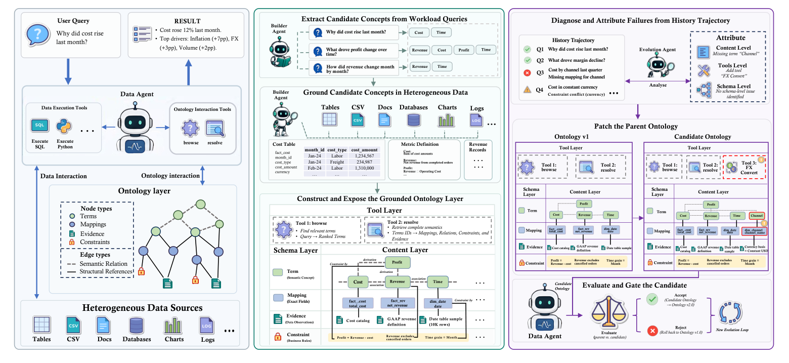
- Profit connects to Revenue and Cost by derivation (Profit is computed as Revenue minus Cost).
- Revenue and Cost each connect to Time by association.
- Cost carries a Mapping that points to
fact_cost.total_cost. - Profit is governed by a Constraint: Profit = Revenue - Cost.
- That Mapping in turn carries Evidence: observed samples of the cost catalog.
The key one is the derivation edge. It makes “Profit does not exist out of thin air; it is computed from Revenue minus Cost” part of the graph structure itself, rather than something buried in a string definition. When the agent looks up the Term Profit, it can follow the derivation edge straight to Revenue and Cost, then follow their structural references to the actual columns and the supporting data. This ability to “walk along relations” is the core difference between a graph and a flat dictionary (such as a traditional semantic layer); the extended reading returns to it.
3.2 Evidence versus Constraint, walked through a card-legality case
Among Term, Mapping, Constraint and Evidence, Evidence and Constraint are the easiest to mix up, because each answers a different question.
| Constraint | Evidence | |
|---|---|---|
| The question it answers | How this concept should be used | Whether claims about this concept are actually true |
| Form | Business-rule text, such as Profit = Revenue - Cost | Actual pieces of data pulled back, such as which values a column really contains |
| Who produces it | The builder agent (the agent that creates the initial ontology) derives the rules from the workload (the set of training queries) and the data | The raw results the builder agent gets by actually querying the data sources |
A real case makes this clearer. Figure 3 shows one accepted patch in a card-legality task, with the added objects marked by red dashed boxes.
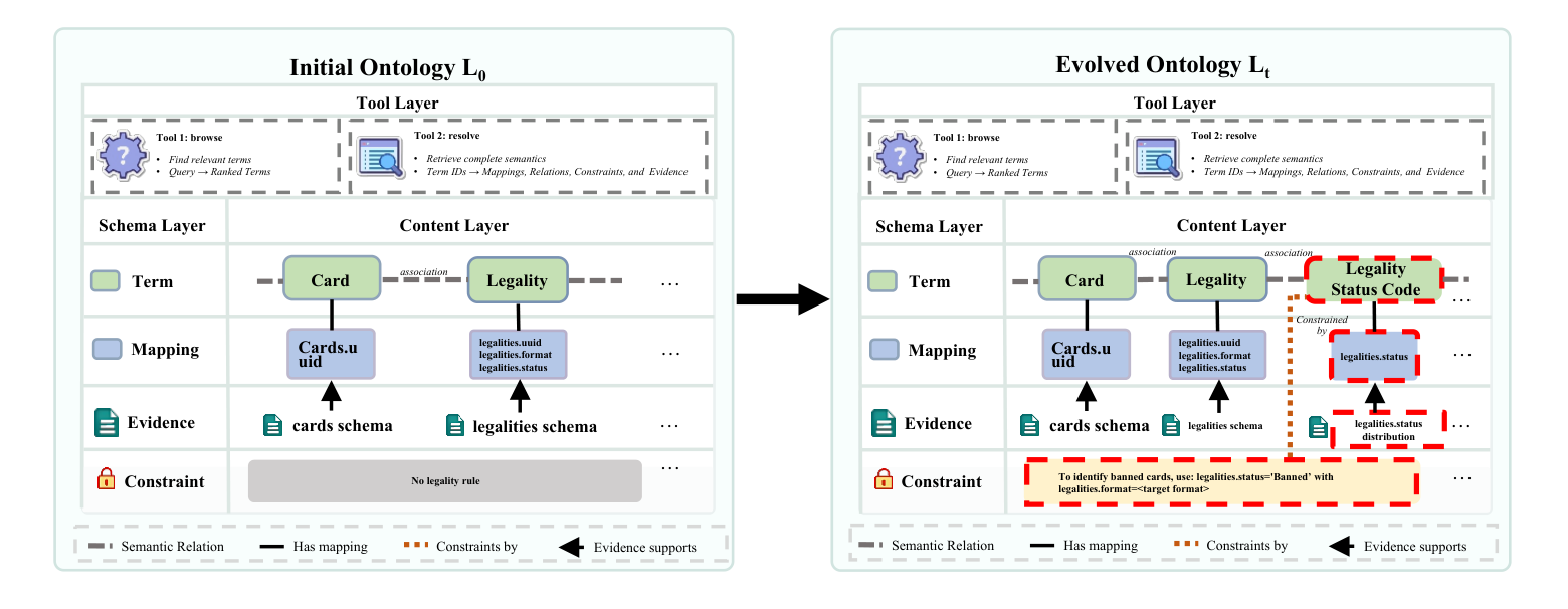
This case lets us walk through it concretely. (How the “accepted patch” in the figure is produced and approved is covered in the section on the self-evolution loop.) The system needs to add the concept “Legality Status Code”, standing for the column legalities.status, and three things go in together:
- Mapping: points to
legalities.status. - Evidence: the value distribution actually observed (Banned, Legal, Restricted and so on).
- Constraint: a card counts as banned only when
legalities.statusisBannedandlegalities.formatequals the target format.
What Evidence does here: the agent does not take on faith that “this column has a value called Banned”; it has really probed the column and has an observation record to point to. Note that Evidence stores more than values. It can also be schema structure, sample data or directory listings (the Content Layer contains schema-observation evidence such as “cards schema” and “date table sample”).
In short: a Term is a concept, a Mapping says which column the concept connects to, a Constraint is the rule for using the concept correctly, and Evidence is the raw observation record proving that these claims have data behind them.
3.3 The Schema Layer: a rulebook like a class definition, and changing it leaves existing knowledge alone
That covers how knowledge is stored; next, the layer that governs the rules. An object-oriented analogy is the most intuitive: the Schema Layer is like a class definition, and the Content Layer holds the objects actually instantiated.
class Term:          # the Schema Layer defines which fields this type has
    name: str
    description: str

term1 = Term(name="Profit", ...)   # the Content Layer holds the actual objects
The Schema Layer defines three specific things:
- The fields of each of the four node families: what a Term, Mapping, Constraint and Evidence each should look like (the paper does not list the full fields of every type; it mentions them only in passing).
- The legal Semantic Relation types: the five listed above.
- The legal reference patterns: which Structural Reference may point at what, for example a Term may connect to a Mapping, and a Constraint may attach to a Mapping or a Term.
The key benefit of this design: changing the Schema does not touch the existing knowledge. Say you want the system to support a new relation type, temporal_dependency (one thing depending on the order in time). You only change . Once the rule exists, the current Profit, Revenue and Cost need no changes at all; they just become describable with the new kind of relation from then on. This also explains why, in the experiments later, Schema-level patches are the fewest: most of the time the problem is missing knowledge content, not an expressive-power limit in the rules themselves.
3.4 The Tool Layer: the agent’s only window, a manifest plus browse and resolve
The first two layers cover how knowledge is stored. This layer covers how the agent gets it, and it is the only one of the three that actually interacts with the agent. The window is made of three things: a manifest, plus two tools, and .
① The manifest. The only thing placed directly in the prompt, and it is very short: which data sources exist and how to use the tools. This answers the problem raised earlier, that a semantic layer hurts because the whole thing goes into the context. Here only the “user manual” goes into the prompt, the actual knowledge stays in the ontology, and the agent decides for itself whether to look something up.
② . Fuzzy matching and retrieval for finding relevant concepts.
| Symbol | Meaning |
|---|---|
| (query) | What the agent wants to look up, in natural language or keywords, such as “cost” |
| (kind) | Which node family to search in: Term? Mapping? Constraint? |
| How many top results to return |
The output is a ranked candidate list: the results semantically closest to .
③ . Fetches the full content of an object you already know.
| Symbol | Meaning |
|---|---|
| The identifier of the object to look up (for example a Term ID obtained from browse) | |
| The paper does not say |
The paper gives only the function signature and, unlike , and , does not explain each parameter. We guess that may be similar to browse’s , limiting which kind of related objects get expanded, but that is only an inference.
The output is the object itself plus everything connected to it (Mapping, Relations, Constraints, Evidence).
3.5 Walking through “Why did cost rise last month?” end to end
| Layer | Role | Can the agent touch it directly? |
|---|---|---|
| Schema Layer | The rulebook: defines which node types exist and which edges are legal | No, it is completely invisible, a gatekeeping mechanism behind the scenes |
| Content Layer | The knowledge itself: the actual graph of Terms, Mappings, Constraints and Evidence | Indirectly, through queries to the Tool Layer |
| Tool Layer | The window: a manifest plus the two MCP tools browse and resolve | Yes, the only interface the agent interacts with directly |
Back to the Figure 2 example. The user asks: “Why did cost rise last month?” and the final result is “Cost rose 12% last month. Top drivers: Inflation (+7pp), FX (+3pp), Volume (+2pp).” The flow in between looks like this:
User    → Data Agent : Why did cost rise last month?
(the manifest is already in the prompt: a short description, no details)
Agent   → Tool Layer : f_browse(q="cost", k="Term", n=3)
Tool    → Content    : semantic matching
Content → Agent      : candidates, Term "Cost" ranked first
Agent   → Tool Layer : f_resolve(I=[Term:Cost], c=...)
Tool    → Content    : follow the edges and pull out the connected objects
Content → Agent      : Mapping / Constraint / Evidence delivered at once
Agent                : builds SQL or Python to query the fact_cost table
Agent   → User       : Cost rose 12%, Inflation +7pp, FX +3pp, Volume +2pp
In short: the manifest tells the agent which windows exist, browse finds the Term, resolve fetches the Mapping, Constraint and Evidence connected to it in one go, and only then does the agent start writing a query.
That was how an already-built ontology gets queried. How the objects in the Content Layer were created in the first place is the next section.
4 Cold start: building the first ontology with no humans and no gold answers
Defining domain concepts, column mappings, join paths and semantic rules by hand takes a lot of expert time. The question here is how the builder agent produces a first version of the ontology automatically, with no human work and without ever seeing the gold answers, using only a set of training queries (the workload) plus the raw data sources.
4.1 Propose, probe, verify, construct: a concept enters only after real data backs it
The process has four steps:
- propose: from the workload , propose a set of candidate concepts , for example Cost, Revenue, Profit, Time.
- probe: for each candidate , actually send probing queries to the data source .
- verify: check whether the probe results match expectations in type, value distribution and semantic consistency; the candidate passes only if they do.
- construct: instantiate the candidates that passed verification into the initial Content Layer, following the Schema Layer’s rules.
The paper describes this with two equations (Equation 1 in the paper). In plain words: only candidates whose probe results pass verification go into , and the Schema’s rules then build them into the initial Content Layer.
| Symbol | Meaning |
|---|---|
| The set of candidate concepts that propose draws from | |
| One candidate in | |
| The result of actually probing the data source for candidate | |
| Checks whether the probe result matches expectations for type, filtering and value distribution; returns 1 if it does | |
| The subset of candidates that passed verification, and the only ones formally admitted into the ontology | |
| Instantiates into the initial Content Layer following the Schema Layer’s rules | |
| The initial Content Layer that gets built |
Here is an illustration rebuilt on the Figure 2 example (the paper itself gives no step-by-step numbers from an actual run):
c = "Cost"
  probe(Cost, D) → finds fact_cost.total_cost, type=number OK, value distribution reasonable OK
  verify(...) = 1 → Cost enters C+, and the samples the probe pulled are stored as Evidence

c = "Revenue", "Time": same process, each passes verification and enters C+
Taken together, propose decides “what to look for”, while probe plus verify decide “whether what was found holds up against real data”, and only after both are done does a concept formally enter the ontology. This is where “evidence-grounded” in the paper’s title comes from.
As for which of these four steps need an LLM, the paper does not say step by step. We worked backward from what each function has to do. Propose has to “understand” the concepts that recur across a batch of natural-language queries, a semantic-understanding task, so it most likely needs an LLM. The part of probe that judges whether “a column name plus sample values really corresponds to a concept” may need one too, but the checks on type and value distribution can be mechanical SQL. Verify, if its rules are clearly defined, can be a plain programmatic condition. Construct just assembles verified candidates into graph nodes following the Schema, which looks like pure engineering. All of this is inference; the paper does not go into this level of detail.
4.2 How the workload is split, and the split-and-swap evaluation
Next, how the data is split. Take a workload of 100 queries. The paper describes only two levels of splitting, and does not separate cold start, evolution and validation into three distinct chunks: the data for cold start and the source of trajectories (the complete record of what the agent did on a task) for the evolution loop are discussed together. So the proportions below are our inference from the paper’s description.
100 queries
   |
   v  first split (assumed close to half-and-half; the paper does not state the exact ratio)
Fold A (about 50) + Fold B (about 50)
   |
   v  second split, only inside Fold A (taking the A→B direction as the example)
70% of A (about 35) → cold-start propose / probe / verify
                      + source of trajectories for the evolution loop
                      (these two share the same batch; the paper does not split them further)
30% of A (about 15) → validation set V for the gate

Fold B (about 50) → never touched; used to compute the final score only after the ontology is frozen

Then run it again the other way, B→A, and finally Score = (Score_{A→B} + Score_{B→A}) / 2
This is called Reciprocal Two-Fold Evaluation (split-and-swap): two disjoint halves of the data take turns as training and test data, and the scores are averaged, avoiding the optimistic bias of “evaluating a system on the same data used to build it”. It is a transferable evaluation methodology, not limited to this paper’s setting.
4.3 The workload-driven blind spot: what was never asked is never learned
Concepts like Cost and Revenue, which map straight onto one column, are easy to probe. But a concept like Profit, which has no physical column and is derived from a formula, raises a question the paper never answers: how is it verified? Going further, propose is purely bottom-up, inferring concepts only from query text, and it does not actively scan the database schema for candidates that “may exist but that the workload never asked about”. This lines up with the schema linking problem in text-to-SQL (mapping the words in a question to the tables and columns of a database); the paper’s own citations, RSL-SQL and E-SQL, are methods built specifically for that sub-problem.
| Workload-driven (the paper’s approach) | Schema-driven (the alternative: hand over the database schema, example queries and domain knowledge) | |
|---|---|---|
| Where candidate concepts come from | Terms that recur in the queries | The database structure itself, plus existing documents and DBA (database administrator) knowledge |
| Advantage | Naturally aligned with real usage, so it will not create concepts nobody uses | Complete coverage: it will not miss columns or concepts that exist in the system but that the workload never asked about |
| Disadvantage | Query patterns the workload does not cover get no matching concept | Prone to creating concepts that are never used; multi-hop join relations still do not resolve automatically |
| When it fits | The workload is representative and covers the main query types | The workload is sparse, or ready-made schema documents already exist; the two can also be mixed |
The paper’s real gap is this: every baseline and every ablation (an experiment that removes one part of a system at a time to see how much the score drops) compares “removing a step inside the workload-driven mechanism”, and no experiment compares against a schema-driven cold start.
There is a mitigating inference, though one with a hole in it (the paper does not say this): the paper’s design philosophy may be not to expect the initialization to be right in one go, but to rely on the later self-evolution loop to patch things afterwards. The hole is that if a complex multi-hop relation is missed at cold start and no user ever asks about it, it never shows up in the execution trajectories either, and the evolution loop has no chance to fill it. This “never asked, never learned” blind spot is likewise not discussed in the paper.
Cold-start summary: a candidate concept must be verified against real data before it enters the ontology, so the first version has evidence behind it; but it infers concepts only from query text, so what was never asked is never learned (this point is our inference).
5 The self-evolution loop: diagnose, attribute, patch, gate
The initial ontology from cold start is a guess based on the workload. Once the agent actually uses it, it will expose “what is missing” and “what is misleading”. The self-evolution loop keeps turning those problems into concrete patches to the ontology. The loop has four steps:
- Diagnose: find recurring failure patterns.
- Attribute: decide which layer the problem belongs to.
- Patch: repair locally, touching only one layer at a time.
- Gate: validate in pairs and decide whether to accept or reject.
Whether accepted or rejected, the loop moves on to the next round and goes back to Diagnose. The paper writes the first two steps up together in one subsection, “Trajectory Attribution”, but its later ablation removes the two steps separately.
5.1 Diagnose and attribute: is the problem in Content, Tool or Schema?
The job is to look back over a batch of records of what the agent actually did on past tasks, find the failure patterns that keep recurring, and decide which part of the ontology fell short: not enough Content, a missing Tool, or a badly designed rule (Schema).
From the paper: “Given historical trajectories and the current state , the evolution agent extracts recurrent signatures . The agent assigns the signature to Content, Tool, or Schema through .”
| Symbol | In plain words |
|---|---|
| Which evolution round; each time a patch is accepted into the ontology, goes up by 1 | |
| The batch of agent execution records accumulated up to round | |
| The complete state of the ontology at round , namely | |
| Takes “this batch of historical records” and “the current ontology” and outputs “which problems keep recurring” | |
| The set of signals that analyze found | |
| One signal in , describing what interaction pattern it is, which ontology objects it involves, and whether it succeeded or failed | |
| The classification function (the blame judge): takes a signal and outputs which layer it is the fault of | |
| The three possible verdicts: Content Layer, Tool Layer, Schema Layer |
Let us run the Figure 2 example through it. The right-hand panel of Figure 2 lists four historical queries as :
Q1: "Why did cost rise last month?"       → ran fine
Q2: "Why did margin decline?"             → ran fine
Q3: "Cost by channel last quarter"        → failed
Q4: "Cost in constant currency"           → failed

analyze picks out two recurring signals:
  σ1 = the question involves "splitting cost by channel",
       but the ontology cannot find a matching Term or Mapping
  σ2 = the question involves "cost at a fixed exchange rate",
       but the agent has no tool for currency conversion

α classifies:
  α(σ1) = Content   (what is missing is the concept itself: a Content-layer gap)
  α(σ2) = Tool      (what is missing is not a concept but a capability: a Tool-layer gap)
The figure also carries the annotation “No schema-level issue identified”: no signal in this round was blamed on the Schema, meaning the existing node types and legal-relation rules are fine and the shortfall is purely content and capability.
The point of classifying “which layer” first is to avoid fixing a problem at the wrong level, for example mistaking a problem of missing tools for one that “just needs a new concept”. How much this design is worth, the ablation numbers later put a figure on.
5.2 Patch: a candidate may change only one layer
For a signal that has been attributed, the system actually builds a repair proposal, under the rule that one candidate patch may touch only one layer.
From the paper: “For an attributed signature , the agent proposes . Each candidate modifies one level only.”
| Symbol | In plain words |
|---|---|
| A signal that has been attributed (for example “the Channel concept is missing”) | |
| The attribution result (for example Content) | |
| The function that generates a repair proposal and outputs a candidate new state | |
| The candidate state; the prime means it has not been formally accepted yet, only proposed, and becomes the official only after validation passes |
What each of the three kinds of intervention may change:
- Content intervention: add, delete or modify the semantic objects already instantiated in the Content Layer (Term, Mapping, Constraint, Evidence, or the edges between them).
- Tool intervention: modify an existing tool, or add or remove tools (), guided by the agent behavior actually observed.
- Schema intervention: modify the Schema Layer’s object model itself, meaning the field definitions of the node types and the legal kinds of relations.
One more point: if a hypothesis needs several mutually dependent Content objects to be fully realized, those objects may be updated together. This does not break “one layer at a time”, because they all belong to the same layer, Content. The card-legality case earlier is exactly that: adding the Term also added its Mapping and Evidence.
Continuing the example, here is what the candidates look like (the “Patch the Parent Ontology” panel of Figure 2: the parent version Ontology v1 on the left, and the Candidate Ontology on the right with two more things than the left):
[σ1: Channel concept missing]      α says Content → patch: add Term:Channel + Mapping (dim_channel.channel_name)
[σ2: no currency-conversion ability] α says Tool    → patch: add Tool 3: FX Convert + Constraint("Currency basis=Constant USD")
These are two independent candidate patches, one touching Content and the other touching Tool. They are never merged into one patch that touches two layers.
5.3 The gate: a candidate must beat its parent by at least τ under identical conditions
A candidate is not the same as an adopted change. The system runs the candidate and the “version before the change” under exactly the same conditions, and the candidate is promoted only if it wins by enough points.
First, one term: backbone means the underlying LLM itself that drives the agent, for example GPT-5.5 or Claude-Sonnet-5. The formula marks the backbone explicitly because the same ontology candidate can perform differently when a different LLM uses it.
From the paper: “For backbone , let denote the score of ontology state on validation set . The candidate and its parent are evaluated on the same with identical decoding and interaction budgets. The candidate is retained only when its improvement reaches margin .”
In plain words: run the candidate and the currently official version on the same validation questions with the same settings. The candidate replaces the current version only if its score beats it by at least ; otherwise nothing changes.
| Symbol | In plain words |
|---|---|
| The scoring function: how well an ontology state does, given the validation set and backbone | |
| The set of validation questions, split off from the training workload and reserved for validation | |
| The candidate version | |
| The parent version (the one currently in force) | |
| The threshold: the candidate must beat the parent by at least this many points to pass | |
| The version in force for the next round |
The point of “paired” is that the candidate and the parent run on exactly the same , with exactly the same sampling settings and exactly the same cap on interaction rounds. With every other variable locked down, any difference in score can only come from what changed in the ontology.
Here is a walk-through with numbers ( is an assumed value; the paper does not disclose the actual threshold):
Candidate 1 (add Channel):    φ(L_t)=70, φ(L'_t)=78, gap 8 ≥ τ(5) → accepted
Candidate 2 (add FX Convert): φ(L_t)=70, φ(L'_t)=73, gap 3 < τ(5) → rejectedHere is how the “Evaluate and Gate the Candidate” panel of Figure 2 is drawn: a balance icon in the middle, and after Evaluate there are two paths. The Accept path promotes the candidate and bumps the version number by one; the Reject path returns to the version before the patch, but it does not stop there: it enters a new Evolution Loop and goes back to Diagnose.
5.4 Candidates are handled one at a time, and rejected ones leave a record
One easily misread point: by the paper’s formulas, candidates are handled one at a time, each round tied to one signal and one candidate. So why can’t several candidates pass at once? Open this up for the paper’s mechanism and the supporting evidence.
You might wonder: if several candidates in the same round all clear the threshold, which one does the system pick? By the paper’s mechanism design, this situation cannot occur. Look back at the formula: patch takes in one and emits one candidate, and the gate compares just that candidate with its parent, one-to-one from start to finish. The formula has no selection mechanism for “several candidates pass at once, pick one”.
There are two pieces of support. First, the caption of the paper’s evolution-round analysis (“Each round corresponds to one candidate that passed the paired gate”) says explicitly that each round corresponds to exactly one candidate that passed. Second, Figure 5 in the experiments: Tool 6 rounds plus Content 11 rounds plus Schema 3 rounds make 20 rounds in all, exactly the total number of accepted rounds, which also supports this reading. So candidates are processed round by round, not competing in a batch:
Round t:   parent=L_t (unpatched) → handle σ1 → candidate L'_t → passes validation → L_{t+1}=L'_t (Channel added)
Round t+1: parent=L_{t+1} (has Channel) → handle σ2 → candidate L'_{t+1} → fails validation → L_{t+2}=L_{t+1} (unchanged)
The parent compared against in the second round is the version that has already absorbed the first round’s patch, not the original version.
What happens once a candidate is rejected? From the paper: “Rejected candidates are not deployed, and their signatures, interventions, and evaluation outcomes are logged to avoid repeated ineffective updates.”
Three things are recorded (continuing the failed Candidate 2 example):
1. signature             → σ2: no currency-conversion ability
2. intervention           → the full content of the candidate "add Tool 3: FX Convert"
3. evaluation outcome     → gap of 3 points, below threshold τ=5, rejected
Why record it? When a candidate is rejected, the problem is actually still unsolved. Without this record, the next round’s analyze may see a similar failure and generate a candidate nearly identical to last time, spend another round of validation on it, and get rejected again, going in circles in the same dead end. With the record, it can in theory steer clear of paths already known to be ineffective.
5.5 Putting the two rounds on one timeline
Looking at the two rounds together shows three things:
- The evolution loop advances round by round rather than competing in a batch, and the parent version is updated with each accepted result.
- The same repair mechanism can succeed or fail.
- A failure is not the end: the problem stays in later trajectories and waits for the next chance.
The whole self-evolution loop boils down to one sentence: first classify where the problem lies, then repair it locally and specifically, and finally let a rigorous paired experiment decide whether to keep the change. It is much like human debugging, except that every step has been formalized into a mechanism that can run automatically.
6 Results: active querying beats stuffing the prompt, and the gate is the step you cannot skip
Now the experiments. Below we keep only the key numbers that carry weight or that change our judgment of the architecture: we did not read the tables closely, judging that the architectural ideas were already clear and the numbers add limited value.
6.1 Main results: all six backbones gain, and stuffing the prompt loses ground
The three benchmarks each test a different capability:
- DDR-Bench: open-ended data research, measuring message-wise and trajectory-wise accuracy.
- InsightBench: business analysis, measuring whether the correct insight is found.
- BIRD: text-to-SQL, measuring query correctness (EX) and efficiency (VES).
DDR-Bench scores are accuracy, higher is better; Message-Wise and Trajectory-Wise are only quoted as numbers in this post, without a breakdown of how they are computed. Also keep two scopes of statistics apart: the main results table (Table 1) covers six backbones, while the +20.0 in the later ablation is an average over just four backbones.
The three conditions compared are: Baseline (no ontology), Baseline+SL (the semantic layer stuffed whole into the prompt), and EvoOntology.
The core conclusion is that EvoOntology beats the Baseline across all six backbones, with an average DDR-Bench gain of +17.8 points (the +20.0 in the ablation later covers a different set, an average over only four backbones, so the two numbers do not contradict each other). Baseline+SL, meanwhile, is often useless or even backslides: Claude-Sonnet-5’s Trajectory-Wise score fell by 15.0 points under Baseline+SL (Table 1). This comparison is the strongest evidence in the whole paper: stuffing everything into the prompt is the wrong road, and active querying is what works.
6.2 Ablations: what the gate, Mappings and the Tool layer each contribute
What each step of the evolution loop costs when removed (DDR-Bench, Traj-Wise, Table 5 in the paper):
| Step removed | Score drop |
|---|---|
| Gate (validation gate) | −11.2 (the biggest drop; without the gate, bad patches get in and cannot get out) |
| Attribution (deciding which layer) | −6.3 |
| Diagnose (finding recurring failure patterns) | −4.8 |
| Patch stage (replaced by free-form rewriting) | −1.7 |
The three editable levels, restricted to one level only (Table 6 in the paper):
| Restriction | Gain |
|---|---|
| Tool layer only | +13.2 |
| Content layer only | +8.7 |
| Schema layer only | +3.6 |
| All three layers open (the full version) | +20.0 |
The three layers complement one another and cannot substitute for each other.
What each object family of the Content Layer costs when removed (Table 7 in the paper; Terms cannot be masked on their own, so they are not in the table):
| Object removed | Score drop |
|---|---|
| Mappings (concept to actual column) | −13.4 (the biggest drop) |
| Evidence (observed support) | −8.7 |
| Constraints (business rules) | −3.5 |
| Relations (semantic relation edges) | −2.1 |
The conclusion: Mappings and Evidence are the real backbone of the Content Layer. Without a Mapping, a concept cannot reach the actual data; without Evidence, the agent has no way to check whether a candidate SQL fragment is right.
6.3 How many rounds of evolution: it varies by backbone and benchmark
The paper never states in its formal experimental setup something like “evolve for N rounds and then score the final version”, but the information is scattered through the Analyses section.
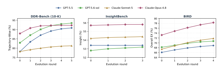
Figure 4 shows DDR-Bench running 0 to 5 rounds, InsightBench 0 to 3 rounds and BIRD 0 to 4 rounds, with different backbones stopping at different rounds. The paper says outright: “GPT-5.6-sol reaching 93.5 Traj-Wise after five accepted rounds and Claude-Opus-4.8 reaching 92.3 after four.”
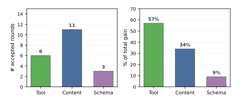
Figure 5 is another clue: summed over four backbones, the Tool layer was accepted 6 times, the Content layer 11 times and the Schema layer 3 times, 20 rounds in all. So the paper does report round counts, but they differ by backbone and by benchmark; they are not a fixed hyperparameter. As for when to stop, the paper says the curves “flatten” over the last two rounds, in its words “the trajectories flatten by the last two rounds, which is consistent with the failure signatures becoming rarer”, yet it does not say whether this is an explicit stopping rule (for example, stop after N consecutive rounds with no passing candidate) or whether the researchers simply stopped running once the trend flattened.
6.4 Transfer across backbones: switch the model and the ontology nearly has to evolve again
This is the finding in the experiments that matters most for “how far this paper is from real deployment”. With the same pipeline, different backbones (GPT-5.5, GPT-5.6-sol, Claude-Sonnet-5, Claude-Opus-4.8) each evolve their own ontology. Take an ontology evolved on backbone A and use it with backbone B, and performance drops across the board, by 6.6 (Sonnet-5) to 10.9 (GPT-5.5) points on average, with no exceptions.
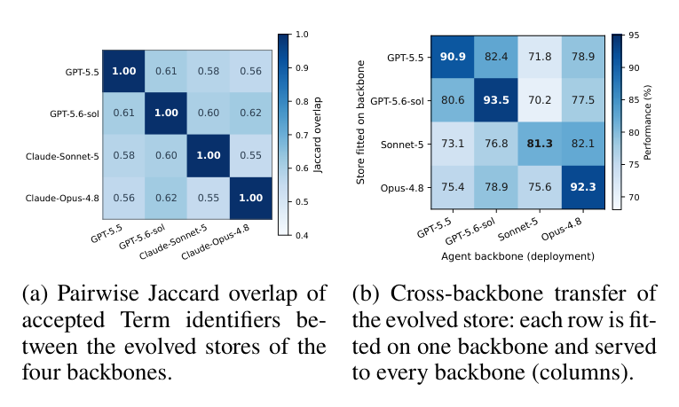
Figure 6(a) shows that the Term sets evolved by different backbones overlap only modestly: the paper notes that no pair exceeds 0.62, and the two Claude models (0.55) overlap even less than the two GPT models do. The implication is direct: this is not a “build once, use everywhere” system. Switching the underlying model means running the evolution again. That is a real cost and limitation at deployment time, and the paper’s abstract does not stress it.
Experiment summary: stuffing the prompt often does nothing or even backslides, and active querying is what works; within the evolution loop the Gate contributes the most (DDR-Bench ablation); Mappings and Evidence are the backbone of the Content Layer; and changing backbone means evolving again.
7 Assessment: a modest, architecture-level contribution with sizable gaps
Overall, the research contribution is modest to low. The core skeleton (a structured knowledge layer, attribution from failure trajectories, a validation gate) matches, in architectural spirit, similar papers on “agent self-evolving knowledge bases or skill libraries” (WikiSkill, for example, another paper in which an agent distills its execution trajectories into reusable knowledge), and is not an original breakthrough. Three contributions hold up relatively well:
- Applying the concrete architecture of “a three-layer split (Schema, Content, Tool) plus MCP packaging” to the agent-data gap, and showing that “active querying beats stuffing everything into the prompt”. Baseline+SL often making things worse is the cleanest evidence.
- The specific design of the backbone-conditional paired validation gate: “candidate against parent, running the same validation set under the same conditions” decides whether to accept a patch, which is relatively rigorous.
- Empirical support from six backbones and three benchmarks, and clear ablations that break down each mechanism’s contribution.
But the ceiling on the contribution is low, because reading all the way through we dug up a long list of places where the methodology is not made clear. These are not trivial details but core engineering details of “whether this system can actually run in practice”:
- Whether cold start and the evolution loop use the same batch of queries, or a further split.
- How the processing order is decided when one round surfaces several signals.
- How the log of rejected candidates affects later patches.
- What the stopping rule for evolution is.
- No experiment compares against a schema-driven cold start, and the “never asked, never learned” blind spot is not discussed.
Another very practical limitation, mentioned earlier: switch to a different LLM backbone and the evolved ontology has to be run again almost from scratch, with no transfer across backbones.
One more point about the name: EvoOntology calls itself an ontology, but it has none of the formal logical reasoning that OWL has (in the fold earlier: a traditional ontology language like OWL can infer automatically, for instance concluding “X flies” from “X is a bird”). Its Content Layer is closer to a queryable typed knowledge graph, oriented toward retrieval, not reasoning. Frankly, the word “ontology” is used a bit loosely here.
8 Takeaways: how much knowledge to stuff depends on its size, and the gate comes first
Even so, the most durable takeaways from this reading are not any of the paper’s numbers but the following ideas, which are connected to one another.
The core principle: whether to hand knowledge to an agent wholesale depends on how much of it there is. The cleanest evidence is that Baseline+SL performs worse than the plain Baseline with no ontology on several backbones, the most extreme being Claude-Sonnet-5 dropping 15 points. The reason is not hard to see: knowledge stuffed statically into the prompt competes for attention with the agent’s other instructions and cannot be trimmed on demand.
That can be abstracted into an actionable rule: for any domain knowledge you give an agent, once there is enough of it to exceed what a single task needs, build it as a tool the agent can actively query and expand on demand, rather than stuffing it unconditionally into the system prompt.
Once knowledge is stored, two organizational questions remain, covered in detail in the extended reading. First, how rules and facts divide the work: an ontology is the rules layer, a knowledge graph is the facts layer, and the rules govern the facts. Second, whether to use flat skill packs or a graph: when domains have derivation or dependency relations (for example Profit derived from Revenue and Cost), a graph only has to define the relation once and it can be followed everywhere; when domains barely reference one another, flat skill packs are enough. These two questions are what unfolds from the same line of thinking about knowledge-supply design, not separate, unrelated points.
The paper’s concrete answer to this problem sits on a more general skeleton: the four-step loop of a self-evolving system. That is diagnose (find recurring failure patterns), attribute (first classify which subsystem the problem belongs to), patch (repair locally, touching only one layer at a time) and gate (paired validation, comparing the candidate with its parent under the same conditions). The value of this skeleton is not that this paper invented it, but that every step has a clear design rationale, and the ablation quantifies each step’s contribution.
Of these, the gate is the one step in the skeleton you cannot skip: without it, any local-repair mechanism can let a bad change into the system, and the system has no mechanism to undo it. For anyone building a system for “an agent that optimizes its own knowledge base or skill library”, this is a priority order you can borrow directly: first make sure there is a rigorous acceptance gate, and only then worry about refining diagnose and attribute.
Finally, the Reciprocal Two-Fold (split-and-swap) evaluation mentioned earlier is the validation framework any scenario in which “the system modifies itself automatically” should adopt: split the data in two halves that take turns as training and test, and average the scores, avoiding the optimistic bias of building and evaluating on the same data.
Back to the main thread: EvoOntology tackles the problem that a data agent does not know its data in advance and has to explore from scratch every time. Its answer is to place a queryable, evolving ontology between the agent and the data, built from three layers: Schema, Content and Tool. The cleanest conclusion from the experiments is that active querying beats stuffing the prompt, and the step in the evolution loop you cannot skip is the validation gate.
The paper’s own originality is limited, and its methodology leaves a number of details unclear; that a new backbone means evolving all over again is a real cost of deployment. Still, the skeleton of “diagnose, attribute, repair locally, validate in pairs”, and the split-and-swap way of evaluating, are worth taking away even apart from this paper.
- Try: next time you prepare domain knowledge for an agent, first estimate how much there is. If it is a lot, build it as a window the agent can query on demand (a manifest plus browse and resolve) instead of stuffing it into the prompt.
- Build the gate first: when you build a self-optimizing system, write the acceptance check that compares a candidate with its parent under the same conditions before you go back to refining diagnosis and attribution.
- Doubt: EvoOntology is a design worth borrowing, not a build-once-use-everywhere system; changing the backbone means evolving again, and details such as cold start and the stopping rule you will have to fill in yourself.
9 Extended reading: a few ideas that hold up beyond this paper
This part collects general ideas that came up during the discussion: questions that were pushed on, clarified, even corrected. They hold up apart from this paper, and they were the most valuable part of this reading. If you only want the paper itself, you can skip this part; the assessment and takeaways above already form a complete conclusion.
9.1 Ontology versus Knowledge Graph: what is the difference?
The corrected framing: both can be graphs, and they differ in the graph’s expressive power and scope.
- Kinds of edges: dbt’s graph has a single semantics, “formula dependency”. EvoOntology’s edges have five semantics (derivation, association, hierarchy, composition, equivalence) and can express a far richer set of relation structures.
- Scope of nodes: dbt’s nodes are limited to metrics and dimensions, tied by nature to structured tables. EvoOntology’s nodes can be any domain concept, and it makes Constraint and Evidence first-class citizens rather than bolted-on annotations.
Now look at how traditional knowledge representation separates an Ontology from a Knowledge Graph:
| Ontology | Knowledge Graph | |
|---|---|---|
| The level it speaks at | The rules layer: defines which classes exist and how classes may legitimately relate | The facts layer: the concrete data points that actually exist |
| Programming analogy | A class diagram or a database schema | The actual rows in the database |
| Logical reasoning? | Usually yes (like OWL) | Usually no; it is just a graph of stored facts |
The relationship between the two: a Knowledge Graph is usually the result of “filling in actual data following the rules of some Ontology”. And EvoOntology’s own architecture happens to contain both layers:
- The Schema Layer is the Ontology half: it defines which node types and which relation types are legal.
- The Content Layer is the Knowledge Graph half: the Terms such as Cost, Revenue and Profit that actually get filled in, and their grounding.
- The former governs the latter.
So calling the paper’s layer an ontology is not misuse: the Schema Layer really plays the role of an ontology in the traditional sense, and the Content Layer is the knowledge graph grown according to those rules.
9.2 Skill-per-domain versus Ontology-graph: how to choose
Many practical agent systems (for example, writing one skill per domain, each skill bound to that domain’s schema and knowledge) fall into the same broad category as this paper’s ontology approach: both structure scattered domain knowledge so the agent can look it up. The difference is in how it is organized.
| Skill-per-domain | Ontology-graph (EvoOntology) | |
|---|---|---|
| Unit of organization | One skill is a complete package for one domain (schema and domain knowledge bundled together) | One Term (concept) is one node, and concepts are linked by typed edges |
| How it is accessed | Tagged by which skill the question maps to | The agent actively calls the two tools browse and resolve; the unit of lookup is a concept, not a whole skill |
| Cross-domain links | Weak: skills are by default unrelated to one another, and crossing domains usually means stitching by hand | Strong: Terms can relate through association, hierarchy, composition, derivation and so on; for example Profit connects straight to Revenue and Cost, and the agent can follow the relations |
The rule of thumb you can carry over:
- When domains barely reference one another (a “document parsing” skill and a “scheduling” skill have little to do with each other, say), a flat skill-per-domain approach is enough and easy to maintain.
- When domains have derivation or dependency relations (a metric that has to combine columns and rules from several different sources, say), the graph structure’s advantage shows, because a relation is defined once and can be followed everywhere, without rebuilding the same derivation logic wherever it is used.
This also connects to the design of self-evolving systems. The earlier ablation shows that removing the gate and attribution costs the most points of all, and they correspond to the core problems any “automatic skill optimization” system must face: how to judge whether a change is really an improvement and whether to accept it, and whether to classify what kind of problem it is before repairing. EvoOntology’s gate design (the candidate and the old version each run once on the same held-out validation set, with the same sampling and interaction budget) is a concrete approach worth consulting; see the Gate section earlier for details.
9.3 Versus WikiSkill: distill then deliver, or query the live structure?
WikiSkill is another self-evolving knowledge-system paper we read earlier. Its architecture has three layers: a Raw Layer (raw trajectories), a Wiki Layer (organized intermediate knowledge) and a Skill Layer (the final skill documents handed to the agent). It tackles the same big problem: how to distill the raw trajectories of an agent’s runs into knowledge that can be reused later. But along one key axis it stands at the opposite end from EvoOntology: whether the intermediate knowledge structure is exposed directly to the agent while it is performing a task.
| WikiSkill: distill first, then deliver | EvoOntology: no distillation, query the live structure | |
|---|---|---|
| How trajectories are handled | Trajectories first go into the maintenance Wiki (the workbench of the optimization process), then get distilled into a Skill (the final product) | Trajectories patch the ontology itself directly (Content, Tool, Schema) |
| What the runtime agent sees | Only the Skill; it never touches the Wiki | It queries the ontology itself through the Tool Layer every time |
WikiSkill’s design is deliberate, not just a temporary training-time limitation: at inference time the agent really does read only the Skill and never touches the Wiki, and this runs through both training and deployment. EvoOntology has no separate “final document” at all: the form of data the agent sees is the same thing as the form the system stores.
This is really the axis one level below the earlier “Skill-per-domain versus Ontology-graph: how to choose” framing: not just how knowledge is organized (a flat pack or a graph) but also how it is delivered to the runtime agent (distilled into one document that exposes only the final product, or letting the agent query the live structure directly with no encapsulation). Each has its merits:
- Encapsulation can keep the agent from being disturbed by the noise of intermediate processes at inference time. WikiSkill’s ablation shows that letting the agent touch the Wiki directly actually lowered final quality.
- No encapsulation keeps the immediacy of “knowledge that is still evolving, with the agent always getting the latest version”, and needs no explicit moment at which “distillation is done”.