Cheap LLM Judge First, GPT-6 Only When Unsure: Does JEV Save Money?

1 Introduction
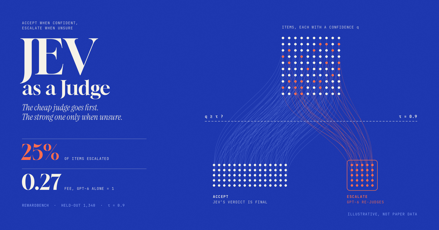
Using an LLM to grade another model’s output (LLM-as-a-judge) has become the default way to run evaluations. The catch is that strong reasoning judges (GPT-6, for example) are expensive and slow, while cheap judges don’t know when they are about to be wrong. This post reads JEV-as-a-Judge: Accept When Confident, Escalate When Unsure (Li, Miao, Krishnan, Padman, Carnegie Mellon University, arXiv 2609.26550v3, September 2026). Its question: if a cheap judge goes first, its verdict is accepted when its confidence is high enough, and only the unsure cases go to the strong judge, can we get close to the strong judge’s accuracy at a fraction of the cost?
This paper is a third-party evaluation, not a new method. Cascading and threshold selection are both established practice. Its value lies in freezing the whole pipeline in advance, validating it on questions it had never seen, and laying out honestly where it works and where it doesn’t. The short answer: it works on tasks where the answer can be read directly from the text. On hard tasks, accuracy holds as long as the threshold is chosen well, but the savings are small.
The post runs in this order: the paper’s problem, the method, the experiments, an overall assessment, “what’s worth taking away”, and finally “concept deep-dives”. The deep-dives cover AUROC, calibration and data splitting, ideas that hold up independently of this paper and last far longer than its specific numbers. When the main text first meets one of these terms, it gives a one-sentence explanation; jump to the deep-dives for the full derivation.
2 30-second version
- Problem: strong reasoning judges are accurate but expensive and slow; cheap judges don’t know when they are wrong.
- Approach: JEV judges every item and its largest label probability is taken as the confidence . If is high enough the verdict is accepted; if it falls below the threshold , GPT-6 re-judges the item.
- Results: on RewardBench the cascade slightly beats GPT-6 in accuracy (+1.27 percentage points) at 27% of the fee. On JudgeBench (harder) and two brand-new tasks it matches GPT-6, but the escalation rate is high (65% to 89%), so the fee savings are only about 9% to 33%.
- Two properties to remember: is good for ranking “which items are more likely wrong”, not for reading directly as “probability of being right”. On tasks with no evidence to check against, confidence fails completely. AUROC measures whether confidence ranks wrong items ahead of right ones; 0.5 is a coin flip, and on that task it was 0.498.
- Verdict: low research value, medium-to-high engineering value within a limited scope. The most portable takeaways are the general ideas around AUROC and calibration, and the line between “answer can be read off” and “answer needs derivation”.
3 Problem and background
3.1 What an LLM judge is
An LLM judge uses one LLM to evaluate another model’s output, for example “which of these two answers is better” or “is this answer supported by the given evidence”. It became the default because human grading doesn’t scale, and automatic metrics like BLEU only match surface text and can’t handle open-ended answers.
Judges come in two kinds:
| Type | How it works | Characteristics |
|---|---|---|
| Reasoning judge | Thinks through a long internal chain before giving a verdict, e.g. GPT-6 | Stronger on hard items, but each judgment costs extra compute: expensive and slow |
| Decision-only judge | Outputs only a verdict and a probability per label, no text | Cheap and fast. JEV (a hosted model from TypeSafe AI; the paper tests version 1.13) is this type |
3.2 Three pain points
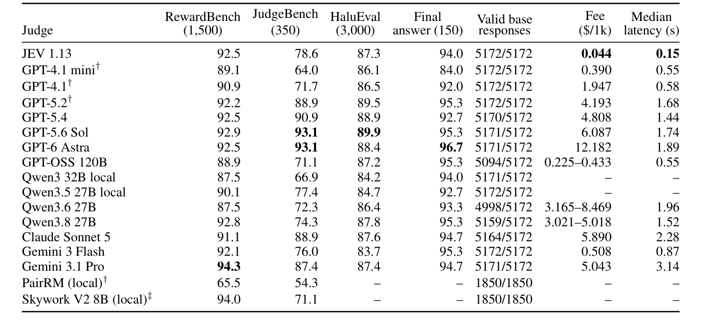
Cost and latency. The paper measures GPT-6 (low reasoning effort) at about USD 12.182 per 1,000 judgments with a median latency of 1.89 seconds; JEV costs about USD 0.044 per 1,000 and 0.15 seconds. That is roughly 277 times cheaper and 13 times faster. The bill is paid again for every new model checkpoint and every new batch of responses.
Confidence is unreliable. If you ask an LLM directly “how sure are you?”, it is often overconfident, assigning high probability even to wrong answers. At scale you need a judge that can tell which verdicts are routine and which need a second look.
Cheap and accurate rarely come together. A single judge forces a choice between the two, so the paper tries to combine their strengths with a cascade.
3.3 How the paper frames the question
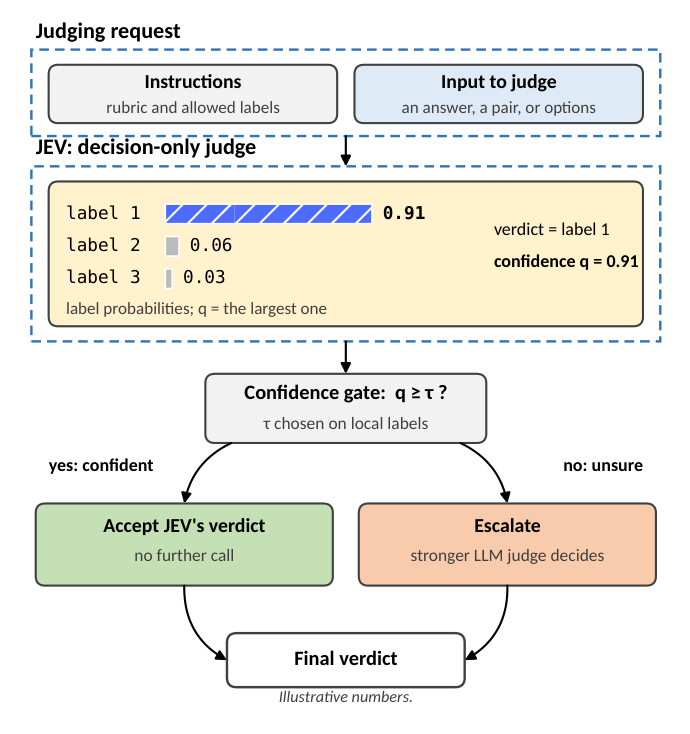
The core idea is the flow chart below: JEV judges every item; if reaches the threshold , JEV’s verdict is the final answer; otherwise GPT-6 re-judges the item independently, and its verdict replaces JEV’s.
So the paper really answers four questions:
- Can JEV’s probability serve as confidence? (Does rank which items are more likely wrong?)
- Is that confidence stable when the presentation order changes?
- How should the threshold be chosen to save the most money while accuracy drops by no more than the tolerance?
- Do these conclusions still hold on unseen items and new tasks?
A note on terms: in this post “escalate” and “defer” mean the same thing, handing an item to the strong judge; “cascade” and “routing” refer to the whole cheap-first, expensive-second pipeline.
The paper measures four things together: accuracy, probability quality (are the probability numbers accurate), fee, and latency.
4 Method
The method has three parts: how to test fairly, how to define and validate the confidence , and how to use to build the cascade and choose .
4.1 Evaluation design
Three kinds of task, ordered from “the answer can be read straight from the text” to “you have to derive it yourself”:
| Task | What is judged | Main datasets |
|---|---|---|
| Pairwise preference | Which of two answers is better | RewardBench (everyday preferences), JudgeBench (harder, correctness can be checked objectively) |
| Evidence-grounded factuality | Whether an answer is supported by the given evidence | HaluEval (hallucination detection) |
| Final-answer verdict | Whether the final answer in a response is correct | 150 multiple-choice responses saved by the authors |
Comparison judges. Besides JEV there are 16 other judges, 17 configurations in total: 14 generative LLMs (including GPT-6, Claude Sonnet 5, Gemini 3.1 Pro) plus 2 reward models (which can’t speak; they only score responses). GPT-6 is the main reference because it is the most expensive and the most stable, and the human review also targets disagreements between it and JEV.
The output contract is the key to a fair comparison. Every LLM judge is required to answer in JEV’s format: one verdict plus a probability per label, with no reasons allowed. That gives every judge the same output shape, so confidences can be compared directly. (Inference: this also limits what a reasoning judge can do, so “GPT-6’s performance” is measured under this restriction.)
Data splits. All 5,172 items are split into 642 pilot items and 4,530 held-out items. “Held-out” means data that is never touched and used only for the final acceptance test. The pilot is further split, by source question, into select (40%, used only to choose thresholds) and test (60%). The rules and the candidate thresholds were fixed before any held-out result appeared. The numbers (in judgments):
| Task | Pilot | of which select | of which test | Held-out |
|---|---|---|---|---|
| RewardBench | 160 | 64 | 96 | 1,340 |
| JudgeBench | 80 | 32 | 48 | 270 |
| HaluEval | 80 | 32 | 48 | 2,920 |
| Final answer and controls | 322 | not split | not split | 0 |
The last row is data the authors prepared separately for final answers and controls; it isn’t split into select/test and has no held-out part (the paper doesn’t give details). What the pilot’s test portion is used for is not stated in the paper; the concept deep-dives discuss it below.
4.2 The confidence q: definition and validation
Definition. is the largest of all JEV’s label probabilities, i.e. how confident it is in the verdict it chose:
- : the probability JEV assigns to label ; the probabilities over all labels sum to 1
- : take the largest one
- In plain words: how sure the judge is of its favourite answer
Example (illustrative numbers from the flow chart): three labels have probabilities 0.91, 0.06 and 0.03, so the verdict is the 0.91 label and .
JEV actually ships a “native confidence” field, but the paper doesn’t use it, for two reasons:
- The other 16 judges only have label probabilities, so using is the only fair way to compare
- TypeSafe hasn’t published the formula for the native confidence
The paper also confirms that the native confidence and rank items similarly (three Spearman correlations of 0.976, 0.999 and 0.958; closer to 1 means more consistent ordering), so switching to loses little.
Pairwise items are asked in both orders and averaged. A judge can be swayed by which answer comes first, so each pair is asked twice; the probabilities are aligned to the same answer, averaged, and the maximum is taken as (HaluEval has no candidate order, so it is asked once).
Made-up example: with A first, JEV says “A is better” with probability 0.90; with B first, JEV says “the first-shown B is better” with probability 0.70, which converts to 0.30 for “A is better”. The average is , so . A judge that favours the first position contradicts itself across the two orders, drops after averaging, and the item is later escalated to the strong judge.
Validation: is actually usable? The paper runs three checks (Section 7 of the paper).
Check 1: is a higher really more accurate? The 4,850 items (original-order judgments from three public benchmarks: RewardBench 1,500, JudgeBench 350, HaluEval 3,000) are grouped by , and JEV’s accuracy is read off per group. For the 214 items with , JEV is right only 55.1% of the time (GPT-6: 69.6%); for the 2,332 items with , both are right 97.8% of the time, right and wrong together, with only 2 exceptions. The gap is concentrated where is low.
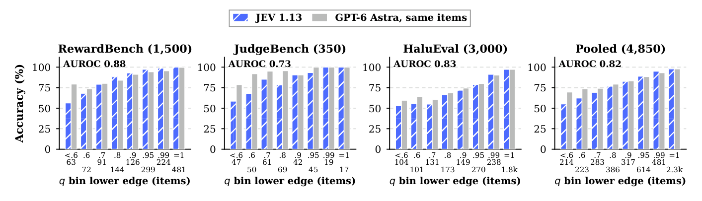
Check 2: can pick out the wrong items? This uses AUROC: sort the items by and see whether wrong items rank ahead of right ones; 0.5 is a coin flip and 1 is perfect (details in the deep-dives below). JEV’s scores 0.88, 0.83 and 0.73 on RewardBench, HaluEval and JudgeBench (two-order average), weakest on the hardest, JudgeBench.
Check 3: is stable when the order changes? JEV had 95 verdict flips after the order was reversed, and only 3 of them happened at . Flips mostly occur on items that were already uncertain.
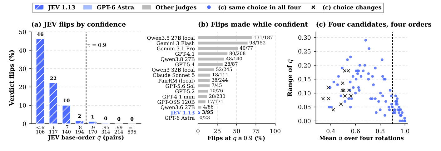
The conclusion you must know: the ranking of can be trusted, the numbers of cannot be read directly as probabilities. Section 7.2 of the paper separates ranking ability (AUROC) from probability quality (Brier score, lower is better; see the deep-dives below):
| Task | AUROC: JEV | AUROC: GPT-6 | Brier: JEV | Brier: GPT-6 |
|---|---|---|---|---|
| RewardBench | 0.875 | 0.894 | 0.113 | 0.115 |
| JudgeBench | 0.745 | 0.907 | 0.297 | 0.095 |
| HaluEval | 0.827 | 0.831 | 0.196 | 0.213 |
The AUROC here is for a single call, so it differs slightly from the two-order-average numbers above. The Brier score is the average squared difference between the probability and the actual right/wrong outcome; lower means more accurate probabilities.
On RewardBench the two are close. On JudgeBench JEV not only ranks worse, its Brier score is three times worse. On HaluEval JEV’s Brier looks better, but the paper points out that this edge doesn’t survive label correction: after humans adjudicated 240 items, the Brier becomes JEV 0.062 versus GPT-6 0.032 (the item count differs so it can’t be subtracted from 0.196 directly, but the direction is clear).
More direct evidence: at the same , the error rate differs by task. It is 1.8% on RewardBench (20 of 1,130 items) and 5.7% on JudgeBench (7 of 123 items; few items, so the number is not very stable).
Calibration can’t rescue this either. Temperature scaling is a knob that flattens or sharpens probabilities as a whole (temperature flattens, sharpens; details in the deep-dives below). The fitted on the three tasks is 0.651, 2.148 and 4.452, inconsistent in direction, and NLL (a probability-quality metric that punishes “very sure but wrong” especially hard; lower is better) actually got worse after calibration on two of them.

So routing uses the relative height of . A threshold can’t be set on the assumption that “ probably means 90% right”; it has to be chosen with each task’s own labelled data.
4.3 The cascade and how the threshold is chosen
The rule. The cheap judge judges all items first, and only the unsure ones go to the strong judge:
- JEV judges every item and gets (for pairwise items, the average over both orders)
- : JEV’s verdict is the final answer
- : hand it to the strong judge, which re-judges independently without seeing JEV’s answer, and its verdict fully replaces JEV’s
is the threshold (the pass line); how to choose it comes next.
Made-up example: 6 items, .
| Item | Goes to | |
|---|---|---|
| 1, 2, 3, 4 | JEV’s verdict is used | |
| 5, 6 | Escalated to GPT-6 |
GPT-6 is paid for only 2 items. But JEV also costs money (twice for pairwise items), so “saving money” compares “JEV on everything plus the escalated items” against “GPT-6 on everything”. That is how the paper computes its fee ratios.
This design works only if the two judges are wrong on different items. Looking at the original-order judgments on all 350 JudgeBench items: JEV is wrong on 75, and GPT-6 gets 60 of those right; GPT-6 is wrong on 24, and JEV gets 9 of those right; 15 items are wrong for both. (The 270 JudgeBench items in the next section are only its held-out part, so the accuracy numbers differ.) With a perfect item picker that chooses the better of the two judges on every item, accuracy could reach 95.7%. Conversely, items both get wrong can’t be fixed however the cascade is routed.
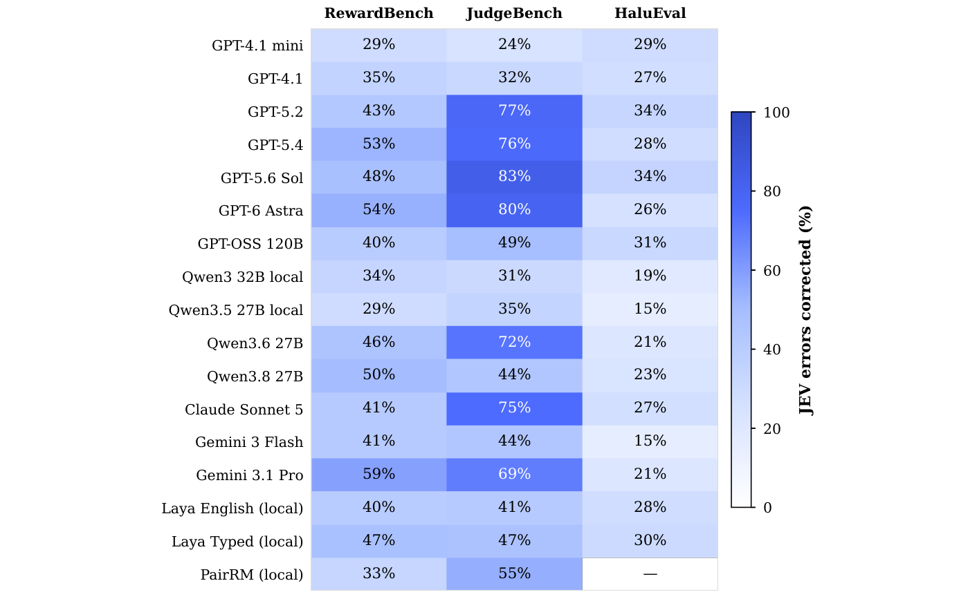
This is only one of many possible designs, and the paper tests only this one (other designs are in the deep-dives below).
4.3.1 Choosing the threshold τ: the basic rule
In one sentence: simulate the cascade on a set of items with ground truth, and pick the that is cheapest while accuracy drops by no more than 2 percentage points.
Think of as a security checkpoint line:
- above the line: waved through, JEV’s answer is used
- below the line: escalated, the strong judge re-judges
- Line set high: many items escalated, high cost, but results close to the strong judge
- Line set low: few items escalated, low cost, but some items JEV would get wrong slip through
For each candidate line, simulate the cascade on the labelled items, compute “share escalated (a proxy for cost)” and “cascade total score”, and compare with the strong judge alone.
Made-up example: 100 practice items, GPT-6 alone scores 90.
| Pass line | Share sent to GPT-6 | Cascade score | Gap vs GPT-6 |
|---|---|---|---|
| 0.99 | 80% | 90 | 0 |
| 0.95 | 55% | 90 | 0 |
| 0.90 | 35% | 89 | 1 |
| 0.80 | 20% | 86 | 4 |
| 0.60 | 8% | 83 | 7 |
The rule: among the lines whose gap to GPT-6 is no more than 2 points, pick the one that escalates least (cheapest). 0.99, 0.95 and 0.90 all qualify, and 0.90 escalates the least, so choose .
The paper’s actual procedure: the candidates are 0.5, 0.6, …, 0.99 (7 values); on the 96 pilot selection items (64 RewardBench, 32 JudgeBench), pick the that stays within 2 points of the strong judge’s selection-set accuracy and accepts the most JEV verdicts (largest coverage), and never refit it afterwards. For GPT-6 this gave .
4.3.2 Choosing the threshold τ: the conservative rule
When practice items are few, a measured “only 2 points worse” may just be luck, so the conservative rule asks “how much worse could it be in the worst case” instead of “how much worse was measured”.
With only about a hundred practice items, the same line could show a gap of 0 on one batch and 4 points on another. The conservative rule (the paper calls it the lower-bound rule) adds a penalty in the bad direction to the measured gap; the penalty reflects how unstable the number is, and is larger when there are fewer items. The result must still be within 2 points to pass.
The paper’s real example (PPE multiple-choice items):
| Pass line | Measured drop | Worst-case estimate after penalty | Passes? |
|---|---|---|---|
| 0.90 | 2.0 points | 4.3 points | No |
| 0.95 | 0 points | not listed in the paper | Yes |
Under the basic rule, just barely passes; the conservative rule sees a worst case of a 4.3-point drop and picks instead. (The penalty of about 2.3 points is my own subtraction of two numbers from the paper.)
General knowledge: this kind of penalty is roughly inversely proportional to the square root of the item count, so going from 100 to 1,000 items shrinks it to about a third. The cost is that the conservative rule usually picks a higher , escalating more items and costing more.
The two rules are used differently in the paper: the main held-out experiment uses the basic rule (96 selection items, giving ); the prospective experiment uses the conservative rule.
The tolerance (how many points of drop you accept) is set by the user, not computed by the model for you. The paper notes that if you know the cost of one wrong answer, the threshold should be derived from “the ratio of error cost to escalation cost”, but it did not test this.
4.4 Putting it together: the full pipeline and a glossary
The whole method chains into six steps:
- Split the data into select and held-out
- JEV judges each item and gets (two-order average for pairwise items)
- Use AUROC to check whether ranks wrong items, and Brier and NLL to check whether the numbers of are accurate
- Choose on select (basic or conservative rule)
- Items with below go to GPT-6
- Validate on held-out
| Term | In one sentence | The question it answers | Which step |
|---|---|---|---|
| Output contract | Every judge returns only a verdict plus label probabilities, no reasons | How to compare fairly | 1 |
| select / held-out | select is for choosing parameters; held-out is never touched and used only for validation | How to avoid fooling yourself | 1, 4, 6 |
| JEV’s probability on its chosen verdict (largest label probability) | How sure JEV is on this item | 2 | |
| Two-order average | Ask pairwise items twice and average, cancelling position bias | Whether is stable | 2 |
| AUROC | The probability that ranks a wrong item ahead of a right one | Whether can rank | 3 |
| Brier, NLL | The gap between probability and actual outcome | Whether the numbers of can be read as probabilities | 3 |
| Temperature scaling | A knob that flattens or sharpens probabilities overall | Whether calibration can be fixed | 3 |
| The pass line; above it JEV is used | How many items to escalate | 4, 5 | |
| Basic rule | Pick the cheapest with a drop of no more than 2 points | How to choose | 4 |
| Conservative rule | Same, but judged by the worst-case estimate | How to choose when items are few | 4 |
Some relationships to remember: the ranking of decides “which items to escalate”; the size of ’s numbers only affects how you interpret them. Temperature scaling fixes only calibration, doesn’t change accuracy, and with two labels doesn’t change AUROC either, so it doesn’t affect routing. is the only knob in this pipeline that truly decides cost and accuracy, and it has to be chosen with the target task’s own labelled data.
Step 3 is actually a diagnostic, not a prerequisite for choosing ; the reason has its own section in the deep-dives below.
5 Experiments
The paper has many experiments; this post keeps the three groups that best answer “can this cascade be used”: the frozen policy on unseen items, the rule not carrying over when the strong judge changes, and the prospective live test. How good itself is was already validated in the section on the confidence q above.
A few terms first:
- Frozen: the rule and threshold are fixed before any held-out result is seen and never adjusted afterwards.
- Offline simulation: the strong judge judges all items first, and afterwards we pretend “only escalated items use the strong judge’s answer” to compute the cascade’s result.
- 95% confidence interval: roughly the range the gap would fall in if you redrew a batch of items. An interval containing 0 means no difference can be seen between the two.
- (delta): the cascade’s accuracy minus the strong judge’s accuracy alone.
5.1 The frozen policy on unseen items
In one sentence: choose on 96 items, switch to 1,610 untouched items, and on the easy task the cascade is both accurate and cheap, while on the hard task it is accurate but saves little.

The table below shows the key columns I picked from the original, which has more columns:
| Task | JEV alone | Cascade | GPT-6 alone | Cascade − GPT-6 (95% interval) | Share escalated | Fee (GPT-6 = 1) |
|---|---|---|---|---|---|---|
| RewardBench (1,340 items) | 92.8 | 93.7 | 92.4 | +1.27 [0.45, 2.03] | 25% | 0.27 |
| JudgeBench (270 items) | 81.3 | 92.2 | 93.0 | −0.74 [−2.22, 0.74] | 65% | 0.67 |
How to read it:
- RewardBench: only 25% of items are escalated, the fee is just 27%, and accuracy is even slightly above GPT-6; the interval excludes 0, so the edge is real. The reason is that the two judges are wrong on different items, so the cascade picks up the best of each.
- JudgeBench: 65% escalated, 67% fee, only a third saved. Accuracy can’t be told apart from GPT-6 (the interval contains 0), but that is thanks to GPT-6 making up the difference.
- Beware the pooled row: the paper has another “all held-out” row (cascade 93.4, fee 0.41), but 83% of held-out is RewardBench, so the pooled row mostly reflects RewardBench; don’t use it to judge hard tasks.
5.2 Same rule, different strong judge: it doesn’t always carry over
Using the same rule to choose , swapping the strong judge gives a different , and on hard tasks it can fail.
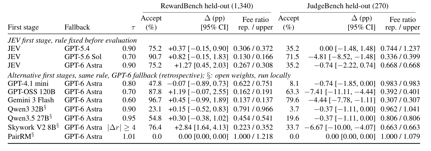
The table below summarizes the original. Three strong judges, same rule, same 96-item selection set:
| Strong judge | Chosen | RewardBench: cascade − strong judge | JudgeBench: cascade − strong judge |
|---|---|---|---|
| GPT-5.4 | 0.90 | +0.37 (interval contains 0) | 0.00 (interval contains 0) |
| GPT-6 | 0.90 | +1.27 (interval excludes 0) | −0.74 (interval contains 0) |
| GPT-5.6 Sol | 0.70 | +0.82 (interval contains 0) | −4.81 [−8.52, −1.48] (interval excludes 0) |
- The first two rows lose no points on either task. GPT-5.6 Sol loses 4.81 points on JudgeBench, beyond the 2-point tolerance, and the interval lies entirely on the negative side, so this is not luck.
- The rule gave it a looser , so on JudgeBench only 28.5% of items are escalated, missing too many items JEV gets wrong.
- The paper’s explanation: only 32 of the 96 selection items are JudgeBench, the rest are RewardBench. Loosening the threshold is safe on RewardBench, and the rule, pulled by that large block, picked a loose that then fails on the hard task.
- Another result: when the strong judge is no more accurate than JEV on the selection set (GPT-4.1 mini, GPT-4.1, GPT-OSS and others), the rule picks , meaning no escalation at all, because escalating brings no benefit.
The takeaway: is not a property of JEV; it is decided jointly by “the first-stage judge, the strong judge and the task”, and changing any of the three means choosing it again.
5.3 The prospective live test
On two new tasks, with the threshold chosen by the conservative rule, the cascade matches GPT-6’s accuracy exactly, but because JEV is already weak on these tasks, only about 25% of the fee is saved.
“Prospective” means writing the rule in stone first and then testing on unseen data, with no chance of adjusting afterwards. “Live” means actually calling the APIs to run the cascade, not simulating offline.
The design freezes the pipeline first, takes 100 items per task as the selection set and chooses with the conservative rule, and then runs the cascade live on the rest. Both tasks were deliberately chosen to be ones where JEV is already weak:
- PPE correctness (500 items): for the same question, the same model produces one correct and one wrong answer, and the judge must tell which is correct
- JudgeBench Claude split (270 items): the group in JudgeBench whose responses were generated by Claude, never judged before
On the selection sets JEV is 12.5 points (PPE) and 17 points (JudgeBench) worse than GPT-6, so the rule chose very strict thresholds: for PPE and 0.99 for JudgeBench.
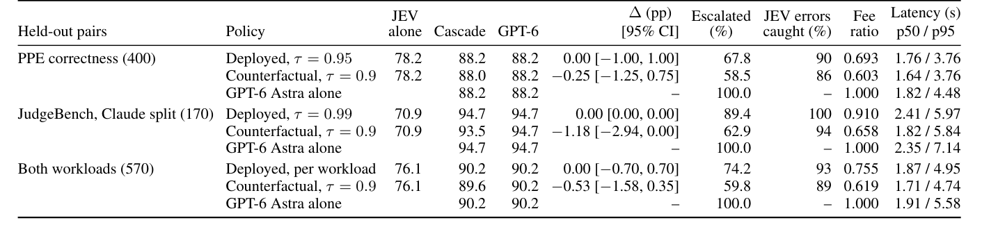
The table below summarizes the original (400 and 170 items are the held-out counts of the two tasks after the threshold was chosen):
| Task | JEV alone | Cascade | GPT-6 alone | Share escalated | Fee (GPT-6 = 1) |
|---|---|---|---|---|---|
| PPE (400 items) | 78.2 | 88.2 | 88.2 | 68% | 0.69 |
| JudgeBench Claude (170 items) | 70.9 | 94.7 | 94.7 | 89% | 0.91 |
| Both combined (570 items) | 76.1 | 90.2 | 90.2 | 74% | 0.76 |
How to read it:
- Accuracy matches GPT-6 exactly: the conservative rule did not choose too loose a threshold on these two tasks.
- But the escalation share is high, and on JudgeBench the saving is only 9%. What the cascade can retain is only the small portion JEV already got right.
- Counterfactual: had the general from earlier been reused (the original has a row for this hypothetical), the fee would fall to 0.62 but accuracy would drop 0.53 points (interval [−1.58, 0.35], contains 0), and 1.18 points on the JudgeBench Claude split. So “choose again for a new task” is validated once more.
- Latency barely improves, see the table below. p95 is the 95th percentile, where the slowest 5% of requests begin. On JudgeBench Claude the cascade is even slightly slower, because escalated items must wait for JEV and then for GPT-6.
| Latency | Cascade | GPT-6 alone |
|---|---|---|
| Both tasks combined: median latency | 1.87 s | 1.91 s |
| Both tasks combined: p95 latency | 4.95 s | 5.58 s |
| JudgeBench Claude: median latency | 2.41 s | 2.35 s |
6 Overall assessment
This is an honest third-party evaluation, not a new method. Its real output is where the “cheap judge goes first, escalate to the expensive one when unsure” pipeline works and where it doesn’t. The engineering value is clearly higher than the research value.
Low research value. Cascading and conservative threshold selection are established practice; the paper itself cites cascade work like FrugalGPT and the 2017 selective-classification literature, and proposes no new algorithm. What counts as contribution is the rigour: freezing the rule before validating, laying out the failure cases (GPT-5.6 Sol, JudgeBench), and drawing the line between “answer can be read off” and “answer needs derivation”.
Medium-to-high engineering value, within a scope.
- Works: tasks where the answer can be read directly from the text. On RewardBench only 25% of items are escalated at 27% of the fee, and accuracy is slightly above GPT-6.
- Fails safe: on weak tasks (PPE, JudgeBench Claude) the cascade’s accuracy still equals GPT-6; the price is spending more (fee 0.69 to 0.91), not losing points.
- Doesn’t work: on tasks with no evidence to check against, ’s ranking ability is a coin flip; don’t use it there.
What the cascade itself brings can be seen in the comparison below (all held-out or prospective experiments, not picked after the fact):
| Scenario | JEV alone | Cascade | GPT-6 alone | Accuracy the cascade adds over JEV (points) |
|---|---|---|---|---|
| RewardBench (1,340 items) | 92.8 | 93.7 | 92.4 | +0.9 |
| JudgeBench (270 items) | 81.3 | 92.2 | 93.0 | +10.9 |
| Prospective, two new tasks (570 items) | 76.1 | 90.2 | 90.2 | +14.1 |
The cascade’s credit is lifting JEV’s weak spots to GPT-6’s level. “Beating GPT-6” appears only on RewardBench (+1.27); JudgeBench doesn’t exceed it, and the prospective experiment is an exact tie.
A few other points call for a discount, so read the numbers for direction only:
- The reference is GPT-6 at low reasoning effort, not at its strongest setting
- Generalization is limited, covering only a few public benchmarks and two new tasks
- The human adjudication (humans re-reviewing items where JEV and GPT-6 disagree with the benchmark label) was not carried out independently
- The paper doesn’t declare the authors’ relationship with TypeSafe (JEV’s provider); the acknowledgments mention only NIST, CMU and OpenAI API credits. The post’s introduction calls this a third-party evaluation, so keep this in mind when reading
7 What’s worth taking away
Saying the engineering value is medium-to-high means this pipeline can be used directly on some tasks. But the paper itself offers little that is new; the durable gains are in the second category. The list below is ordered by durability, most durable first.
7.1 Category 1: the paper’s own contribution
7.1.1 A reproducible cascade pipeline with prospective validation
The pipeline: average the two orders, choose on labelled items, escalate only items with low , and validate on untouched items. It isn’t a new method; the paper’s value is that it freezes the whole pipeline in advance and tests it on two new weak tasks, where accuracy matches GPT-6 at a fee of 0.69 to 0.91. The lesson to take: this pipeline doesn’t lose points on weak tasks, it just saves little.
7.1.2 The boundary of applicability measured for JEV 1.13
On tasks where the answer can be read from the text, JEV is within 2 points of GPT-6; on tasks that need derivation or checking it trails by 7 to 28 points; on tasks with no evidence to check against, confidence fails completely. This boundary was measured for a specific version and may move when a new version arrives, but the split “a judge’s strength depends on whether the task is reading or deriving” itself holds (see item 4 in Category 2).
7.1.3 The specific numbers are the least durable
JEV’s accuracy and GPT-6’s fee and latency are tied to specific model versions, reasoning effort and pricing at the time; they will go stale fast, so there’s no need to memorize them.
7.2 Category 2: what holds beyond this paper
7.2.1 Evaluate a “classifier that gives confidence” along three independent dimensions
Accuracy looks at whether the verdict is right; AUROC looks only at the order of ; Brier and NLL look at the size of ’s numbers. These measure different things, so a judge can be very good on one and very poor on another.
| The question | What to look at | What happens without it |
|---|---|---|
| Is the verdict right | Accuracy | Everything else is moot |
| Can rank who is more likely wrong | AUROC | Can’t use confidence to pick items |
| Can ’s numbers be read as probabilities | Brier, NLL | Confidence numbers mislead |
A concrete example is in the AUROC and Brier sections below: two judges rank identically, both with AUROC 0.78, but one is honest in its confidence and the other overconfident, so their Brier scores differ a lot.
The use decides which metric to look at: if you only need the verdict, look at accuracy; if you use confidence to pick items to re-check (routing, human review), look at AUROC; if you read confidence as a probability (risk estimates, combining with other systems), look at Brier and NLL.
7.2.2 Calibration moves only the numbers, not the ranking, and calibration is tied to the task
Temperature scaling divides the logit difference by and converts back to a probability. With two labels the new confidence is an increasing function of , so the order of items and the verdicts don’t change:
- : the difference between the two labels’ logits (the model’s raw scores), taken as positive
- : temperature, a positive number; gives the original probability, flattens it, sharpens it
- In plain words: divide the score gap by first, then convert to a probability the usual way
Made-up example: (). With , . Every item is flattened, the order is unchanged, so accuracy and AUROC don’t change; only Brier and NLL change.
The paper’s numbers are Table 2 above: for the same JEV, RewardBench fits (NLL goes from 0.192 to 0.216, worse), JudgeBench (0.449 to 0.475, worse), and HaluEval (0.496 to 0.304, better). The directions are inconsistent, and on two of the tasks calibration actually makes things worse.
In practice: for routing alone you don’t need calibration, since good enough ranking is all that matters; to read as a probability, calibrate separately with “that task’s own labelled data”.
7.2.3 A cascade’s value comes from “the two judges being wrong on different items”
The result of a cascade is that accepted items use the first stage’s answer and escalated items use the strong judge’s answer. If the strong judge gets most of the first stage’s wrong items right, escalating repairs them. But items both get wrong can’t be repaired however they are routed.
Made-up example: 100 items, the strong judge is wrong on 10, JEV on 15, and 3 are wrong for both. With a perfect item picker that escalates only the items JEV would get wrong, the only remaining errors are those 3, so cascade accuracy is 97%, higher than the strong judge alone at 90%. If the two judges’ errors were identical (all 15 overlapping), the best the cascade could do is the strong judge’s level.
The paper’s real numbers were listed in the cascade section above (JudgeBench 350 items: JEV wrong on 75, GPT-6 wrong on 24, 15 wrong for both); a perfect picker reaches 95.7%, above GPT-6 alone at about 93%.
When choosing a first stage, look at:
- Beyond being cheap, whether its errors differ from the strong judge’s, and how many items its lets you wave through (cheap but almost nothing waved through saves no money)
- A cascade’s ceiling is the errors shared by both, not the strong judge’s own accuracy
- The more alike two judges are (same family, same training data), the less useful the cascade (inference, not directly tested in the paper)
7.2.4 Whether a judge is usable: first ask “can the answer be read off or checked”
A judge’s job is comparing, not solving from scratch. If the answer can be read straight from the text, a small model is enough; if you have to re-derive the answer to know whether it is right, a small model falls short.
Made-up example: “Does this response refuse the user?” You know after one read; “Does this program have a bug?” You have to run it in your head.
The paper’s numbers: on tasks where the answer can be read off, JEV is within 2 points of GPT-6. On tasks that need derivation it trails by a lot: knowledge −7.0, code −12.9, math −14.3, logic puzzles −27.6 (JEV minus GPT-6 accuracy, in percentage points).
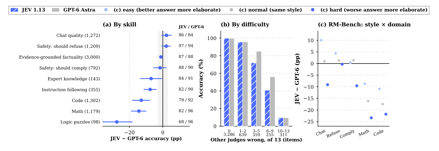
Before going live: sort your tasks into three kinds. Answer can be read off: a cheap judge is enough. Needs derivation: expect to escalate a lot to the strong judge. No evidence to check against: see the next item.
7.2.5 High confidence doesn’t mean reliable, especially when the judge has nothing to check against
A model’s probability reflects “how sure it is of its own output”, not “how close the answer is to the facts”. When the judge has no evidence to check against, it will still give a very confident answer.
The appendix has direct numbers: on 200 responses with no evidence to check against, a binary choice where a coin flip gets 50%, all three judges are close to a coin flip yet all very confident. JEV’s AUROC is 0.498, so confidence can’t tell right from wrong at all.
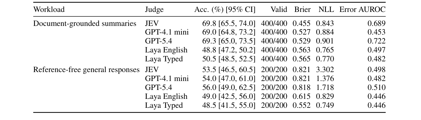
| Judge | Accuracy | Mean top probability |
|---|---|---|
| JEV | 53.5% | 0.91 |
| GPT-4.1 mini | 54.0% | 0.94 |
| GPT-5.4 | 56.0% | 0.96 |
Checks before going live:
- Confidence routing assumes “low-confidence items are more likely wrong”, so measure AUROC on labelled items first to verify it
- When AUROC is close to 0.5, don’t route by confidence; escalating won’t help either, because the strong judge is also close to guessing
- Limitation: only 200 items, and the paper itself says it can only show that the result depends on the task, not that the difference comes purely from having evidence. Details in the “reference-free responses” section below
7.2.6 When designing a cascade, look at “what failure looks like”: a good design fails by costing more, not by losing points
A cascade’s safety comes from one structure: low goes to the strong judge, so the more uncertain the first stage, the more is escalated and the closer the final answer gets to the strong judge alone. When the first stage gets weaker, the system pushes cost up instead of letting errors through.
The prospective experiment (Table 5) supports this: on two tasks where JEV was already weak, accuracy still matched GPT-6 exactly, at the price of a fee close to GPT-6 alone (PPE: 68% escalated, fee 0.69; JudgeBench Claude: 89% escalated, fee 0.91).
This guarantee has two limits:
- It holds only when the threshold is chosen right. The paper’s counterexample: GPT-5.6 Sol’s was set to 0.70 and it lost 4.81 points on JudgeBench.
- On tasks with no evidence to check against, the strong judge is itself close to guessing and escalation won’t improve things, so the “failure means costlier” guarantee doesn’t hold there either.
Design principle: for any routing or escalation mechanism, ask two questions. When the first stage fails, are errors let through, or is cost pushed up? When the threshold is set wrong, which side breaks? A good cascade design should make the cost side the only thing that breaks when the threshold is set conservatively.
8 Concept deep-dives
Each section here can be read on its own and holds up independently of this paper.
8.1 Data splitting: what the rest of the pilot is for
The paper splits the 642 pilot items into select (40%) and test (60%). Select is used to choose thresholds, so what is the test 60% for?
The paper doesn’t state a separate use for the pilot test portion. I found no result in the main text or appendix where it appears on its own; the validation of temperature scaling and the acceptance of thresholds both use held-out, not pilot test.
What the paper does say: the pilot is frozen before any model inference; select is used only to fit temperature and the routing threshold. “Source-cluster” means repeated responses to the same question stay on the same side, so one question doesn’t end up in both select and test. The numbers are the table in the earlier “Evaluation design” section, in judgments. The pilot’s 642 = select 128 + test 192 + the unsplit 322.
My inference (not the paper’s wording): the pilot test portion probably has no separate role and is just folded into the overall accuracy in Table 1. The evidence is that RewardBench’s 160 plus 1,340 add up exactly to Table 1’s 1,500, which means all pilot items (select and test) count toward the overall accuracy.
One consequence of this split: select’s 128 items also count toward Table 1’s accuracy, so those numbers aren’t a perfectly clean held-out result. But 128 of 5,172 is small, so the effect on the conclusions is limited and it isn’t a serious flaw.
The general idea is why data is split into different roles:
| Role | What it does | Why it must be separate |
|---|---|---|
| select | Decides parameters, such as the threshold and the temperature | This data has already been “seen”; it is used to choose parameters |
| held-out | Used once, at the end, for validation | Must have had no part in the choice, or the number can’t be trusted |
Data used to choose parameters can’t also be used to prove the parameters were chosen well. Example (made up): you pick the that gives the best accuracy on a batch of items, then report accuracy on that same batch. Of course the number looks good, but it only proves “this fits this batch”, not “this fits new items”. Keeping validation items completely separate is the only way to know what happens on items you haven’t seen.
8.2 AUROC: understanding it by lining up
AUROC asks just one thing: line all the items up by from low to high; do the wrong items stand ahead of the right ones?
Its full name is Area Under the ROC Curve, and here it measures “how well ranks wrong items”. In plain terms: the probability that, when you draw one wrong item and one right item at random, the wrong one has the lower . 0.5 is a coin flip and 1 is perfect.
Made-up example: 6 items; JEV is wrong on 3 and right on 3, and each has a . First line them up by from low to high:
| Rank | Actual | |
|---|---|---|
| 1 | 0.55 | Wrong |
| 2 | 0.60 | Right |
| 3 | 0.70 | Wrong |
| 4 | 0.90 | Wrong |
| 5 | 0.95 | Right |
| 6 | 0.99 | Right |
If were a perfect wrong-item detector, all 3 wrong items would stand at the front. In reality the 2nd place is a right item, mixed in among the wrong ones.
To turn “how well ranked” into a number, pair every wrong item with every right item, 3 × 3 = 9 pairs, and for each pair ask only “does the wrong item have a lower than the right item?”
| Wrong item’s \ right item’s | 0.60 | 0.95 | 0.99 |
|---|---|---|---|
| 0.55 | ✓ | ✓ | ✓ |
| 0.70 | ✗ | ✓ | ✓ |
| 0.90 | ✗ | ✓ | ✓ |
7 of the 9 pairs are ranked correctly, so AUROC = 7 / 9 ≈ 0.78.
A feel for the numbers (general knowledge, not from the paper):
| AUROC | The feel |
|---|---|
| 0.5 | is unrelated to right or wrong, like rolling dice |
| 0.7 | Somewhat useful, but the ability to rank wrong items is shaky |
| 0.8 to 0.9 | Practical level, most wrong items rank ahead of right ones |
| 1.0 | Perfect, practically never seen |
AUROC looks only at order, not at the size of . Change every in the table above to 0.01, 0.02, 0.03 and so on: as long as the order stays, AUROC is still 0.78.
The consequence of this blind spot (made-up example): take the same 6 items, where the actual accuracy is only 50%. Judge X’s values are 0.55, 0.60, 0.70, 0.90, 0.95, 0.99; Judge Y’s are 0.950, 0.960, 0.970, 0.980, 0.985, 0.990. The two rank identically, and both have AUROC 7/9. But Judge Y claims over 95% confidence on every item while being right only half the time. AUROC can’t see the difference at all; that takes a metric like Brier (see “How to measure calibration” below).
Back to the paper: on HaluEval, GPT-6 and JEV have nearly identical AUROC (0.831 versus 0.827), yet their Brier scores differ (0.213 versus 0.196). Same ranking ability, different probability quality. (Though, as the earlier section on confidence noted, this Brier gap doesn’t survive label correction; it is used here only to show that “Brier can differ when AUROC is the same”.)
The paper’s numbers (single-call AUROC) are the first two columns of the table in the earlier section on confidence. On RewardBench and HaluEval, JEV’s ranks wrong items about as well as GPT-6. JudgeBench is the point: GPT-6 scores 0.907 and JEV 0.745. This is the hardest set; GPT-6 is not only more accurate, it also better “knows when it will be wrong”.
For a classifier that gives confidence, AUROC answers only “can rank who is more likely wrong”. It doesn’t answer “does really mean 90% right”, nor “is the verdict right”. The three have to be looked at separately.
8.3 What routing becomes when AUROC is low
A low AUROC means it’s hard to know which items to hand to the expensive judge, so you pay more or accept more errors, but it is not “escalate everything”.
Routing exists to “pick out the items likely to be wrong and send them to the expensive judge”. With a high AUROC, escalating only a few items catches most of the errors; with a low AUROC you have to escalate many to catch them, and the savings shrink.
A low AUROC doesn’t mean you can only send most items to the expensive judge. In direction you do have to escalate more, but in practice you are trading off between “how many to escalate” and “how many errors to let through”; a low AUROC just makes that trade more expensive.
Made-up example (rough, only to show the direction): of 100 items, 10 are ones JEV would get wrong.
| High AUROC (about 0.9) | Low AUROC (about 0.6) | |
|---|---|---|
| Want to catch 8 wrong items | Escalating about 20 items is enough | May need to escalate 60 or more |
| Escalate only 20 items | Catches about 8 wrong items | Catches only about 3 to 4 wrong items |
When AUROC is low you have two options: pay more (escalate more items), or accept more errors (escalate the same number and let more wrong items through). “Escalate everything” is the most extreme of these choices.
The paper’s measurement: at threshold , 1,106 of the 4,850 items (about 23%) were escalated, and the other 3,744 used JEV’s answer directly. That 23% is the trade-off point chosen “under JEV’s ranking ability”.
8.4 Calibration: the probability says 90%, is it actually 90%?
Calibration means that among the items where the model says “90% sure”, about 90% are really right:
- : the confidence the model gives
- : a specific confidence value, such as 0.9
- Left side: among all items whose is exactly , the share where the verdict is correct
- In plain words: items with confidence 0.9 should be right 90% of the time
Made-up example: Judge Y says on all 100 items but is right on only 50. Ideally 96 would be right, but only 50 are, so Y is overconfident. Conversely, saying 0.6 and being right 90% of the time is underconfident.
Ranking and calibration are two independent properties:
| Well calibrated | Poorly calibrated | |
|---|---|---|
| Ranks well | Ideal | Can rank wrong items, but the numbers can’t be read directly |
| Ranks poorly | Honest numbers, but no help | Both fail |
Evaluating a classifier that gives confidence takes at least three independent questions: accuracy for whether the verdict is right, AUROC for whether can rank who is more likely wrong, and calibration metrics (Brier and the like) for whether ’s numbers themselves can be trusted. A judge can be very good on one and very poor on another. AUROC covers only ranking; calibration metrics are in the next section.
8.5 How to measure calibration: reliability curve, Brier, ECE, NLL
There are several common tools for measuring calibration, differing in whether you want to see “where it’s off” or “how much it’s off in total”.
8.5.1 Reliability curve: seeing where it’s off
Group items into bins by the size of and compute one point per bin; the curve is those points joined up:
| What to compute | How | Plotted on |
|---|---|---|
| Mean confidence | The average of over all items in the bin | x-axis |
| Actual accuracy | Items right in the bin ÷ total items | y-axis |
With perfect calibration every point lies on the diagonal.
Made-up example: 10 items with the and outcomes below, cut into 3 bins.
| Bin | in the bin | Mean confidence | Right | Accuracy |
|---|---|---|---|---|
| 0.5 to 0.7 | 0.52, 0.58, 0.63, 0.67 | 0.60 | 2/4 | 0.50 |
| 0.7 to 0.9 | 0.72, 0.78, 0.85 | 0.78 | 2/3 | 0.67 |
| 0.9 to 1.0 | 0.91, 0.96, 0.99 | 0.95 | 3/3 | 1.00 |
The three points are (0.60, 0.50), (0.78, 0.67), (0.95, 1.00).
There are two ways to cut the bins (general knowledge, not from the paper):
| Equal-width bins | Equal-count bins | |
|---|---|---|
| How | Every bin has the same width, e.g. 0.0 to 0.1, 0.1 to 0.2… | Every bin has the same number of items; boundaries are set by the data |
| Pro | Simple, the x-axis is easy to read | Every point has similar reliability |
| Con | Items often pile into a few bins while others have only a few, so points jitter | The range of in one bin can be wide |
A rule of thumb: when the distribution of is concentrated at one end, use equal-count bins, or cut the crowded end finer.
The paper’s reliability curves are in the bottom row of the figure below. The caption says only “a bin needs at least 5 items to be plotted”; how the boundaries are cut isn’t stated. Figure 2 earlier has unequal-width boundaries (<0.6, 0.6, 0.7, 0.8, 0.9, 0.95, 0.99, =1), cut especially fine at the high-confidence end, because JEV’s piles up near 1 ( alone has 2,332 items).
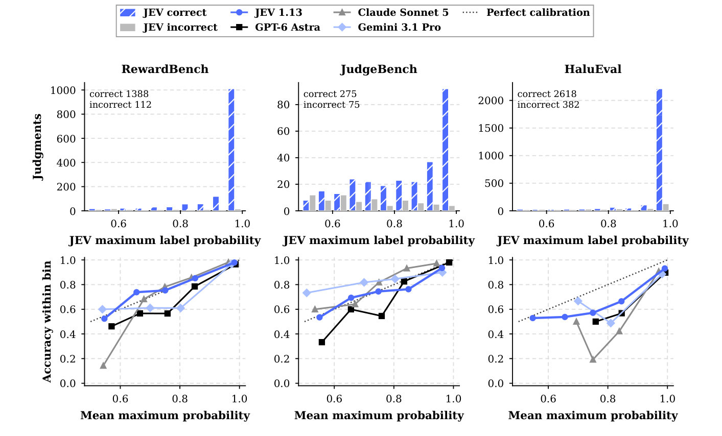
8.5.2 Brier score: how far off in total, as one number
- : the confidence on item
- : the actual outcome on item , 1 if right, 0 if wrong
- : the number of items
- In plain words: square each item’s “confidence minus outcome” and average; lower is better
Made-up example: reuse the 6 AUROC items. Judge X’s values are 0.55, 0.60, 0.70, 0.90, 0.95, 0.99 and the outcomes are wrong, right, wrong, wrong, right, right, so Brier . Judge Y’s values are 0.95, 0.96, 0.97, 0.98, 0.985, 0.99 with the same outcomes, giving Brier . The ranking is the same (AUROC 0.78 for both), but Brier differs a lot.
This is a simplified version that looks only at whether is right. The paper’s Brier is computed over the probabilities of all labels, so the details differ slightly.
8.5.3 ECE (expected calibration error): compressing the reliability curve into one number
- : the number of bins
- : the number of items in bin ; : the total number of items
- : the actual accuracy in bin
- : the mean confidence in bin
- In plain words: compute how far off each bin is, weight bins with more items more heavily, and add them up
Computed on the 10-item reliability-curve example above:
| Bin | Items | Mean confidence | Accuracy | Gap | Weight (items ÷ 10) | Contribution |
|---|---|---|---|---|---|---|
| 0.5 to 0.7 | 4 | 0.60 | 0.50 | 0.100 | 0.4 | 0.040 |
| 0.7 to 0.9 | 3 | 0.78 | 2/3 | 0.113 | 0.3 | 0.034 |
| 0.9 to 1.0 | 3 | 0.95 | 1.00 | 0.050 | 0.3 | 0.015 |
ECE 0.089, meaning the average deviation is about 9 percentage points.
Two design choices are worth noting: taking the absolute value keeps “overconfident” and “underconfident” from cancelling out; weighting by item count is because bins with few items are unreliable to begin with. ECE’s drawback (general knowledge) is that its value changes with how the bins are cut.
How the paper uses it: the main text relies mostly on Brier and NLL; the appendix also reports ECE (with 10 maximum-probability bins). Why the main text didn’t choose ECE isn’t stated in the paper.
8.5.4 NLL (negative log-likelihood): punishing “very sure but wrong” especially hard
For each item, take “the probability the model gives the correct answer”, compute , and average over all items; lower is better.
| Probability the model gives the correct answer | |
|---|---|
| 0.9 | 0.11 |
| 0.5 | 0.69 |
| 0.1 | 2.30 |
| 0.01 | 4.61 |
The difference from Brier: a judge that is 99% sure but wrong has given the correct answer only 0.01. Brier’s penalty for that item is at most 1 (a square can’t exceed 1), while NLL’s is 4.61, and as approaches 0 it keeps climbing with no upper bound. So NLL is especially strict on “very sure but wrong”, and Brier is gentler. The paper reports both so as to look at probability quality from two angles.
8.6 Why models are often poorly calibrated
Nothing in training forces the model’s probabilities to tell the truth, and some training steps even push it toward overconfidence. What follows is general knowledge, not from the paper.
Reason 1: the training objective rewards only “getting it right”, not “honest probabilities”. An analogy: an exam looks only at whether you picked the right option, and nobody checks the “how many tenths sure am I” you wrote beside it, so over time you have no reason to learn to write that down accurately.
The underlying mechanism: a classification model converts raw scores (logits) into probabilities (softmax) at the end. The cross-entropy loss used in training (which is really NLL) keeps rewarding the model even when it is right, because “the correct answer’s probability hasn’t reached 1 yet”. Made-up example, two classes’ logits:
| Logits (correct class, wrong class) | Probability of the correct class | Loss when right |
|---|---|---|
| [2, 0] | 0.881 | 0.127 |
| [4, 0] | 0.982 | 0.018 |
Both cases have the right verdict, but the second has lower loss. So training keeps widening the score gap, pushing probabilities ever closer to 1, though the probability of being right doesn’t really rise with it. This is the phenomenon pointed out by Guo et al. 2017 (which the paper also cites): modern deep networks are generally overconfident.
Reason 2: post-training pushes probabilities to extremes. A pretrained model’s token probabilities are usually fairly honest, but after training such as RLHF, which targets human preference, the output is pushed toward “sounding certain”.
Reason 3: calibration holds only “for one kind of item”. Probabilities tuned well on type-A items drift on type-B items, because the model’s difficulty and error patterns differ across items. The paper’s direct evidence is in Section 7.2: for the same JEV and the same temperature-scaling procedure, RewardBench fits (sharpening the probabilities), while JudgeBench and HaluEval give and (flattening them).
8.7 With two labels: q and the logit gap, temperature scaling, and why accuracy and AUROC don’t change
With two labels, is determined by a single number, “the gap between the two scores”; temperature scaling divides that gap by as a whole, so verdicts and the order between items don’t change, only the probability numbers do. What follows is for the two-label case (the paper’s main task) and is general knowledge unless noted.
8.7.1 The relationship between q and the logit gap
A logit is the model’s raw score for each label, and softmax converts them to probabilities. With two labels:
- , : the logits of the two labels
- : their difference, written
- In plain words: the absolute size of the two scores doesn’t matter, only the gap decides the probability
Be careful with JEV: the paper never mentions logits and doesn’t say how JEV produces its probabilities internally, so “whether JEV’s probabilities come from a logit gap” is not stated in the paper. But you don’t need to know: given a probability you can back out , which is called the log-odds:
Made-up example: a judge says on some item, .
8.7.2 How temperature scaling works
- Take the probability
- Convert it to the score gap
- Divide by
- Convert back to a probability
- Try many values of on the selection set and pick the one that minimizes NLL
- Validate on held-out
flattens the probability, making it less confident; sharpens it, making it more confident; is the original probability.
Made-up example, logits [4, 0] (), with the correct class’s probability as varies:
| Score gap after dividing | Probability of the correct class | Effect | |
|---|---|---|---|
| 0.5 | 8 | 0.9997 | Sharpened, more confident |
| 1 | 4 | 0.982 | Original |
| 2 | 2 | 0.881 | Flattened |
| 4 | 1 | 0.731 | Flattened further |
In plain words: a judge says 0.982 on a whole batch of items but is actually right on only 70%. brings the probability down to 0.731, close to the true 0.7, so lands somewhere around there. (The actual fit minimizes NLL over all items rather than matching one number.)
The paper fits on the select set and validates on held-out (Table 2). Step 2, backing out from the probability, is my inference; the paper doesn’t say how it actually scales JEV.
8.7.3 Why accuracy and AUROC don’t change
There are two different levels of ordering here, and they must not be mixed up:
| Metric | Why it doesn’t change |
|---|---|
| Accuracy | The verdict takes the label with the largest probability. Every score is divided by the same , so which label is larger doesn’t change, and the chosen label doesn’t either |
| AUROC | It looks at the order of across different items. With two labels is an increasing function of , and changing only flattens or lifts it as a whole, so the order between items doesn’t change |
Made-up example: 3 items whose logit gaps are 0.5, 1.5 and 3.0.
| Item | at | at | |
|---|---|---|---|
| A | 0.5 | 0.623 | 0.562 |
| B | 1.5 | 0.818 | 0.679 |
| C | 3.0 | 0.953 | 0.818 |
Going from = 1 to 2, every item’s moves toward 0.5, but the order A < B < C is unchanged. So if the wrong items were ranked first before, they still are, and AUROC doesn’t change.
After adjusting , accuracy and AUROC stay the same, while Brier, NLL and ECE change (all three measure “are the probability numbers accurate”). Temperature scaling fixes only “calibration”, which is exactly the benefit of accuracy, AUROC and the calibration metrics each handling one thing.
8.8 Is validating q a necessary condition for choosing the threshold?
The method has a “validate whether is useful” step (AUROC, Brier, NLL), but as long as there are the two steps “simulate the cascade on labelled items and choose ” and “validate on held-out”, it seems you can already choose the best threshold, so why validate ?
For “choosing ”, validating is not necessary. Simulating the cascade measures the final outcome directly (how much it costs, how many points are lost), which already contains the information on whether is useful. Validating is a diagnostic, not a prerequisite.
What validating adds:
| What validating adds | Can simulating the cascade give it? |
|---|---|
| Why it fails: is the ranking poor, or the probabilities off? | No. Simulation only tells you “no passes” or “one passes” |
| Judging whether the task is worth cascading at all | Partly. For example, for reference-free responses with AUROC 0.498, simulation would also end in “escalate everything”, but you’d have to run both judges first to know |
| Reusable when the strong judge changes (inference, not stated in the paper) | No; with every new strong judge the simulation has to be redone |
The first is the main value. The second saves only a little cost: AUROC needs only the first-stage judge to have run, with ground truth, and doesn’t pay for the strong judge.
Brier and NLL are even less necessary. Routing uses only the ranking of and never reads as a probability, so they don’t affect how is chosen at all. They are useful when you want to report as a “probability of being right”, compare probability quality with other judges, or do something else that needs probability numbers.
The engineering judgment:
- To choose : you need only “simulate the cascade” and “validate”
- Treat AUROC as a cheap pre-screen; Brier and NLL can be skipped
- The paper validates so thoroughly because it has to answer the research question “on which tasks does this approach work”, which is research value, not a deployment requirement
One reservation (inference): when the labelled data for choosing is very small, the result is unstable (see the conservative rule in the cascade section), and AUROC can then serve as a cross-check. The paper doesn’t validate this use.
8.9 What kinds of cascade design exist, and which ones the paper tested
The paper tested only the “independent, replace” design; the other two were not validated, so it can’t be called the best. The paper’s own wording is that fusion, letting the strong judge see JEV’s verdict, and building the correlation of the two judges’ errors into the rule are all left for future work (end of Section 7).
All three designs are “cheap judge goes first, escalate to the strong judge when unsure”; they differ in how the strong judge is used:
| Design | How | Drawback and source |
|---|---|---|
| Independent, replace (the paper’s choice) | The strong judge doesn’t see JEV’s answer and simply replaces it | Items the strong judge also gets wrong can’t be repaired (the paper’s own words) |
| Let the strong judge see JEV’s verdict | More information, like a debate | The two judges’ errors become dependent on each other (the paper’s own words) |
| Both judge everything, then fuse | Average the probabilities | The strong judge is paid for on every item, so no money is saved (my inference; the paper didn’t test fusion or compute its fee) |
What the paper actually compared is something else:
| Comparison | What it answers | Can it show “this design is best”? |
|---|---|---|
| Random escalation at the same fee (the grey line in Figure 7 below) | Is picking items by better than picking at random | No, it only shows is useful |
| Different strong judges (GPT-5.4, GPT-5.6 Sol, GPT-6) | Does the design still hold when the judge changes | No, the design didn’t change |
| Different first-stage judges | Is JEV especially suited as a first stage | No, the design didn’t change |
All three comparisons are fixed under “independent, replace”. So what the paper can support is that, under this design, routing by works, not that “this design is better than the others”.
My view (inference): this design is the simplest, cheapest and easiest to deploy, but “simplest” doesn’t mean “best”. Whether to switch to another combination can only be decided by testing on your own data.
8.10 What “reference-free” means and why confidence fails
“Reference-free” means the judge receives only “a question plus a response”, with no evidence document or ground-truth answer to check against, and must rely entirely on its own knowledge to decide whether the response is making things up (hallucinating). On this kind of task JEV’s is neither accurate nor able to tell what to hand to whom.
Made-up example for comparison:
| With evidence to check against | Reference-free | |
|---|---|---|
| What the judge gets | A document and a one-sentence summary | Only a question and a response |
| What is asked | Is the summary supported by the document? | Is this response making things up? |
| How the judge decides | Checks the summary against the document | Can only guess from what’s in its head |
The paper’s numbers are in Table 6 and the small table below it: on 200 reference-free general responses, binary choice, all three judges are close to a coin flip yet very confident (mean top probability 0.91 to 0.96). JEV’s Brier is 0.821 and its AUROC 0.498, which means can’t tell at all which items will be wrong.
This breaks the cascade, because routing assumes “items with low are more likely wrong”. Here is high everywhere, and its height is unrelated to right or wrong, so no threshold can pick out the items to escalate. And even if you escalate, the strong judge GPT-5.4 gets only 56%, so it’s no use. The paper concludes that “none of the tested judges can be used on this kind of item”, so this is not a JEV-specific problem.
Limits to keep in mind:
- Only 200 items, with a 95% confidence interval of [46.5, 60.5]
- The paper itself says this set differs from the evidence-grounded one in both content and label source, so it can only say “the result depends on the task”, not that the difference comes purely from having evidence
The general idea: confidence reflects how sure the model is of its own output, not how close the answer is to the facts. When a judge has nothing to check against, it will still give a very confident answer, so before going live always measure AUROC on labelled items to verify whether confidence is any use.
8.11 The cost and accuracy trade-off of a cascade
Every cascade has a trade-off between cost and accuracy, even randomly handing items to the strong judge. What the paper really wants to show is: picking items by is better than picking at random, and you can know in advance on which tasks it holds.
Even with a high threshold you can still save a little. In Table 5’s JudgeBench Claude split, with and 89.4% of items escalated, accuracy is exactly the same as GPT-6 (94.7%) and the fee is only down to 0.91.
Using the strong judge directly is the most stable baseline, but not necessarily the fastest:
- Most stable: the most accurate option is to use the strong judge directly
- Latency: escalated items wait for JEV and then for GPT-6; JudgeBench Claude’s median latency of 2.41 seconds is even slower than GPT-6 alone at 2.35 seconds
That picking by beats random can be seen in the post hoc sweep below. It is read off the same items, so it is optimistic: at the cascade scores 90.2%, while random escalation at the same fee gets only 89.0%. The shape of the curve is the point, not the trade-off itself.
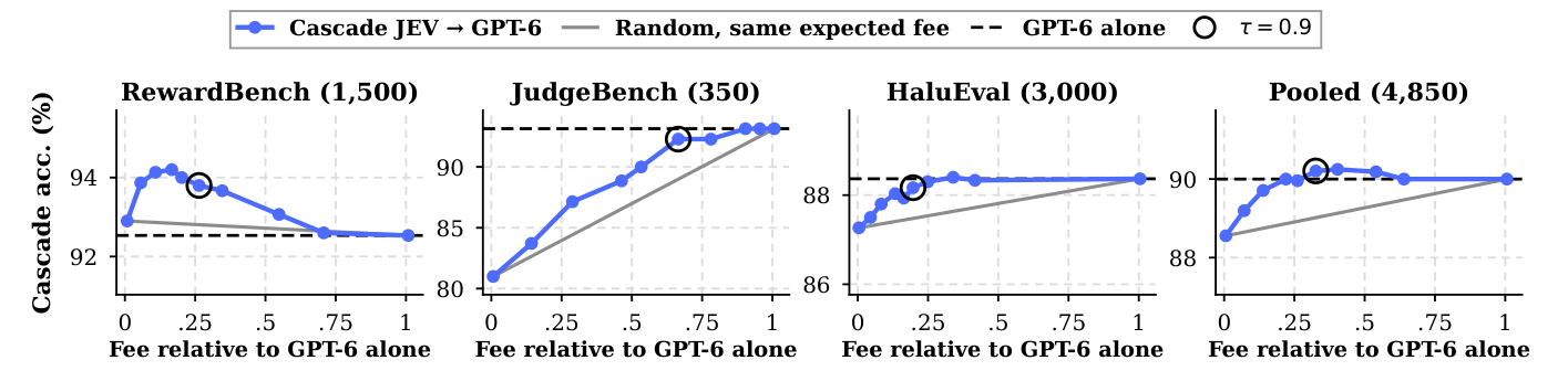
Choosing the threshold looks like mere exhaustive search, but the difficulty isn’t in the search. is a single parameter with only 7 candidate values, so exhaustive search is cheap. The real difficulty is that when labelled items are few, the measured drop is very unstable, which the paper handles with the conservative rule (see the cascade section). The rule isn’t a new method, the tolerance is set by a person, and there’s no statistical guarantee; the paper mentions that if the cost of errors is known the threshold should be derived from the cost ratio, but didn’t test it.
9 Conclusion
This paper proves one thing within a scope: using JEV’s largest label probability as confidence and routing by “accept when confident, escalate to GPT-6 when unsure” is both accurate and cheap on tasks where the answer can be read from the text (RewardBench: 27% of the fee, accuracy slightly above GPT-6); on hard tasks and new tasks, accuracy holds when the threshold is chosen right, but the savings are limited (9% to 33%).
A few points to remember: is suitable only for ranking, not for reading as a probability; is a function of the first-stage judge, the strong judge and the task, and changing any of them means choosing it again with your own labelled data; on tasks with no evidence to check against, confidence fails completely, so don’t use it there. The specific accuracy and fee numbers will go stale quickly; what lasts is the division of labour between AUROC and calibration, the discipline of splitting data, and the design principle that “a good cascade fails by getting costlier, not by getting wronger”.