More Examples Isn't Better: Rethinking Many-Shot CoT-ICL

1 Introduction

Long-context models let us stuff dozens or even hundreds of examples into a prompt for In-Context Learning (ICL). On simple tasks like classification and intent detection, the industry has accumulated two rules of thumb that feel like common sense: more examples are better, and order barely matters. The paper “Many-Shot CoT-ICL: Making In-Context Learning Truly Learn” asks a pointed question: when the examples themselves carry Chain-of-Thought (CoT) reasoning, and the tasks become multi-step problems like geometry proofs and number theory, do those two rules still hold?

Not really, it turns out. The authors find that Many-Shot CoT hits a series of counterintuitive failures on reasoning tasks — performance gets less stable as you add examples, picking the “most similar” examples as references is actually a trap, and the influence of ordering explodes as the example count grows. In response, the paper proposes two design principles — example content must be “understandable,” and example ordering must be “smooth enough” — and operationalizes the second one with an ordering algorithm called CDS (Curvilinear Demonstration Selection). These notes follow that same thread, laying out the paper’s core findings and how CDS actually works.

2 A Paradigm Shift: ICL Isn’t Copying Answers, It’s Real-Time Learning at Test Time

To understand why the old rules fail, you first have to grasp the authors’ redefinition of ICL.

Traditionally we treat long context as a static retrieval buffer: the model finds the examples in the prompt whose surface features most resemble the current problem, then “copies” the answer format across. That logic works well for classification, since classification only requires recognizing the distributional features of labels. But the authors argue that when facing complex reasoning, Many-Shot CoT is actually much closer to gradient-free real-time adaptation — the prompt is no longer just reference material, it’s a training signal the model uses during the forward pass to dynamically shape its internal problem-solving procedure. This “the model learns as it works at inference time” framing runs along the same line of thought as the test-time learning idea in Dynamic Cheatsheet, which we’ve covered before.

Another way to see it: the traditional approach is like handing a student a cheat sheet full of past exam questions. During the exam, if the wording matches, they copy the answer straight across — good enough for easy problems. But for complex math reasoning, one change of problem type or one different number and it’s useless. What the student actually needs is a “cram-session workbook” — pitched close to their current level of understanding, with problems arranged in a progression.

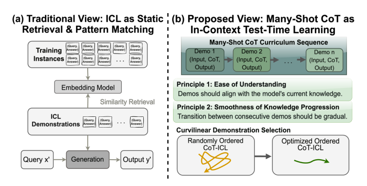
This shift to an “educational” perspective leads directly to the paper’s two core design principles: content must be comprehensible, and ordering must be smooth. The next section looks at what goes wrong when you don’t follow them.

3 Three Counterintuitive Findings: Where Many-Shot CoT Actually Breaks

3.1 More Examples, More Confusion

By the old rules, going from 16 examples to 128 should steadily improve performance. The paper does observe that trend on non-reasoning tasks (SuperGLUE, BANKING77). But switch to reasoning tasks like geometry, number theory, or GSM8K, and the accuracy curve starts oscillating violently — and in some cases clearly declines.

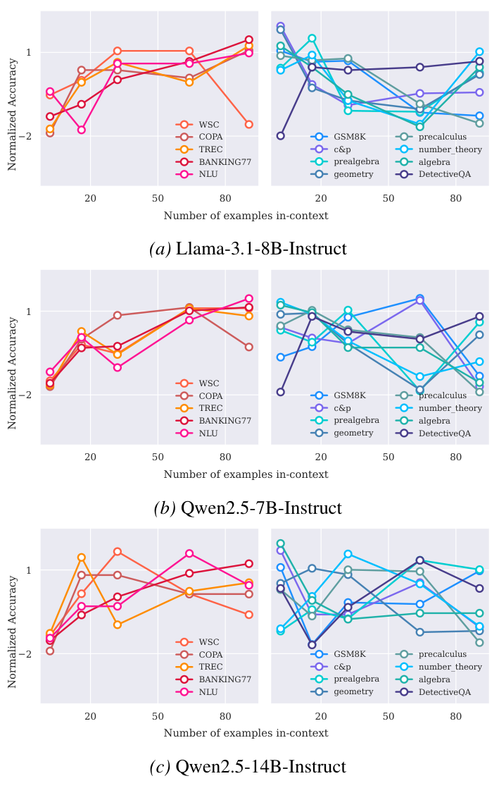
At first this negative scaling looks like a symptom of insufficient model scale, but the authors find that even at LLaMA 3.3 70B, adding examples still yields negative returns. The real dividing line isn’t scale, it’s model type: “reasoning models” like QwQ and DeepSeek-R1 — trained with explicit reasoning mechanisms built in (producing <think> tokens, for instance) — actually improve steadily with more examples on the very same tasks.

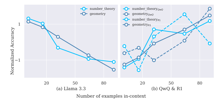
This isn’t hard to picture: take an average student, hand them a hundred-page problem book full of complex geometry proofs, and give them no guidance whatsoever. They won’t suddenly have a breakthrough from reading a few more pages — they’re more likely to get tangled up in the sheer volume of information and start botching even the easy problems they could previously solve.

3.2 Picking the “Most Similar” Examples Is a Trap

The gold standard in traditional RAG is semantic similarity retrieval — find the examples that most resemble the test question on the surface, since those are the easiest for the model to imitate. But the paper finds that on reasoning tasks, the most similar examples are often poison.

The problem is that “semantically similar” is not “procedurally compatible.” Take an example from the paper: two geometry problems both mention a right triangle with 30°-60°-90° angles, making them extremely similar semantically — but one requires proving a side-length relationship via triangle similarity, while the other needs the Pythagorean theorem and an area formula to find an altitude. If the model copies the first problem’s solution steps to solve the second, the logic simply doesn’t line up, and the whole thing falls apart.

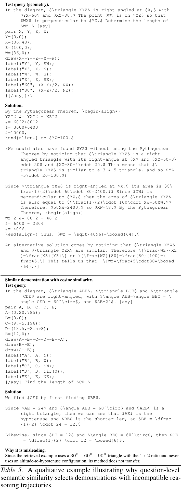
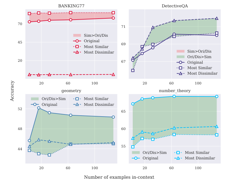
In Section 4.3, the authors run a controlled comparison: on non-reasoning tasks, the “most similar” examples perform best; but on geometry, number theory, and DetectiveQA, “most similar” consistently underperforms both “least similar” and random selection. The reason is that semantic similarity is only a weak proxy metric — it offers no guarantee that the solution procedure of the example is compatible with that of the test question.

3.3 With More Examples, Ordering Matters More, Not Less

By the old rules, once you have enough examples, randomly shuffling their order should have almost no effect — this is “order robustness.” The paper measures accuracy standard deviation across 5 different random orderings, and classification tasks do follow the old rule: more examples, smaller standard deviation, more stable model. Reasoning tasks do exactly the opposite — standard deviation grows explosively as examples are added.

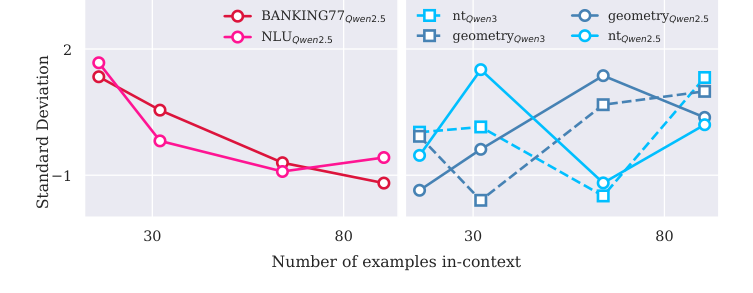
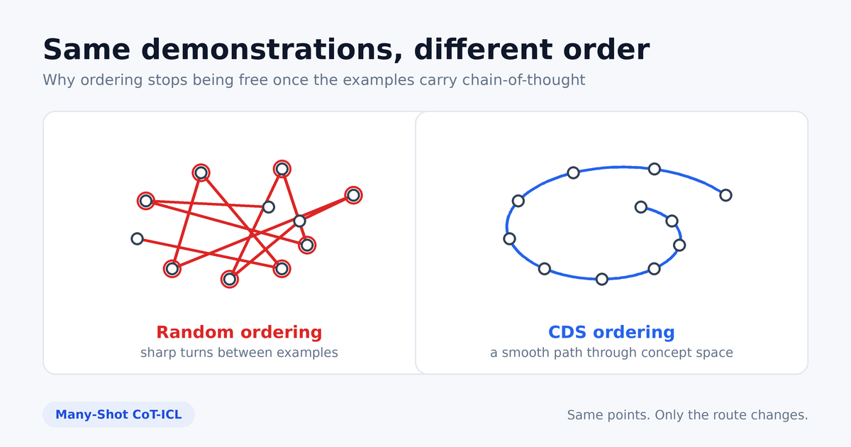
This means Many-Shot CoT exhibits clear “path dependence” — randomly shuffling a hundred reasoning examples is like a textbook with chaotic chapter ordering, teaching addition on page one, jumping to calculus on page two, then back to subtraction on page three. These conceptual hairpin turns send the model’s reasoning trajectory ricocheting back and forth, and the more examples there are, the higher the odds of hitting one of these “logical cliffs.”

4 Principle One: Examples Should Be “Understandable,” Not “Well-Written”

The fix for the first challenge comes from the “Zone of Proximal Development” concept in educational psychology: the most effective teaching material isn’t the most difficult textbook, but the material that falls within what the student “can understand with appropriate guidance.”

The paper maps this onto language models as “Distributional Alignment”: the closer an example’s linguistic style, reasoning step size, and logical structure are to the target model’s own output distribution, the more easily the model internalizes those reasoning steps. Put bluntly, the human-written reference answers in a dataset are like a textbook written by a university professor — logically polished, but with large conceptual jumps that an 8B model may not be able to digest. The chains of thought the model generates itself, by contrast — clumsily written, sometimes even miscalculated — are in “the same distribution’s language,” and the model actually learns from them faster.

To test this hypothesis, the authors had LLaMA 3.1 (8B) use three different example sources on reasoning tasks: the dataset’s reference answers (origin), the model’s own correctly-solved examples (cr), and the model’s own incorrectly-solved examples (wr). The result is quite surprising: whether the answer was right or wrong, any self-generated CoT consistently beat the reference answers.

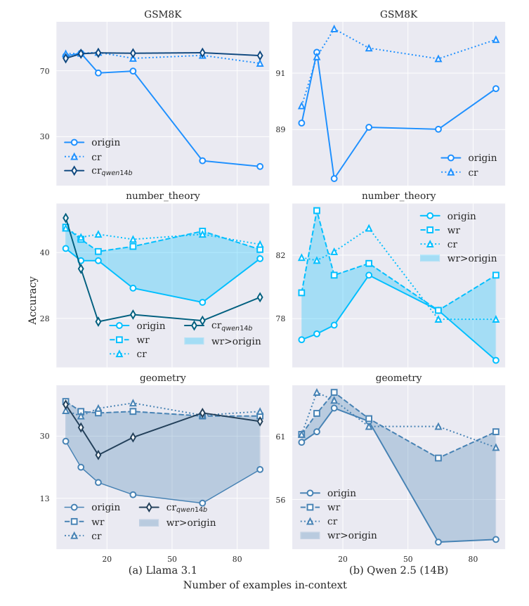
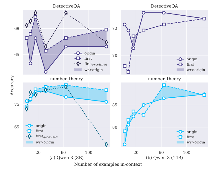
In other words, what the model genuinely absorbs during ICL is “procedural supervision” — the logical framework and steps of solving the problem — not rote memorization of the final answer’s digits. This advantage shrinks as model scale grows, because a model with stronger comprehension is better able to see through the semantic structure of a difficult reference answer; and the reasoning models mentioned earlier, like Qwen 3 and DeepSeek-R1, also show higher resistance to misaligned reference answers.

5 Principle Two: CDS — Turning Ordering into a Journey Without Hairpin Turns

With “what content to pick” settled, the next problem is “how to order it.” This is the paper’s weightiest contribution: the CDS (Curvilinear Demonstration Selection) algorithm.

5.1 Example Ordering as a Journey Through High-Dimensional Space

Feed each example (question + chain of thought + answer) into an embedding model and it becomes a point in high-dimensional space. With 100 examples you have 100 points, and ordering them is essentially finding a single continuous route through all 100. If the route keeps making hairpin turns and doubling back through concept space, the model’s reasoning gets muddled; if the route is smooth and the transitions between concepts are natural, the model absorbs it cleanly.

This maps neatly onto a classic optimization problem: the Traveling Salesperson Problem (TSP) — visit every city exactly once, return to the start, and minimize total distance. TSP is NP-hard; 100 cities means 100! possible permutations, so in practice you rely on heuristics to find a “good enough” solution in reasonable time rather than solving for the global optimum. In the CDS setting, the cities are the examples, the route is the ordering, and the fare is “the comprehension burden of reading the next example after the previous one.”

5.2 The Cost Function: Distance and Turning Angle Together

In CDS, the cost of moving from example $i$ to example $j$ has two components:

$\delta_{ij}$ is the Euclidean distance between the two points, ensuring that adjacent examples progress gradually in concept space rather than jumping between problem types; $\gamma_{ij}$ is a curvature proxy cost, meant to quantify whether the path makes a hairpin turn.

There’s a technical subtlety here: to judge whether the path turns sharply at point $j$, you theoretically need to know the direction of both the previous step ($i \to j$) and the next one ($j \to k$) — but at the time you place $j$, the algorithm has no idea what comes next. The authors’ solution is to find the candidate example closest to “the geometric midpoint of $i$ and $j$” and treat it as the “anticipated next step $k(i,j)$,” then use an inner product to compute the angle between $i \to j$ and $j \to k$. The sharper the turn, the higher the curvature cost.

5.3 The Four-Step Workflow: Greedy Init → Local Search → Multi-Start → Cut the Loop

CDS in practice breaks down into four steps:

1. Greedy initialization (Nearest Neighbor): pick a random starting point, then at each step choose the lowest-cost next point until the loop closes, producing an initial tour — though this tour usually has plenty of self-crossing “knots.”
2. 2-opt local search: repeatedly check for cheaper connections, eliminating crossings by reversing subsequences to smooth the route out.
3. Multi-start (Random Restart): local search easily gets stuck in local optima, so rerun from different random starting points, up to 10 times, and keep the route with the highest smoothness score.
4. Cut the longest edge: TSP produces a closed loop, but a prompt is a straight line — so the final step finds the single most abrupt, longest-span edge in the route and cuts it, turning the loop into a sequence with a beginning and an end.

The 2-opt step deserves a closer look, since it’s where the algorithm actually performs surgery. Say the current ordering is [0, 1, 2, 3, 4, 5, 6, 7, 8, 9] (with the last point connecting back to the start). The algorithm uses a nested loop to pick two non-adjacent edges, say 0→1 and 4→5. It looks up the total cost of both connection schemes in the cost matrix: the original Cost(0,1) + Cost(4,5), versus the reversed Cost(0,4) + Cost(1,5). If the reversed version costs less, it flips the entire segment from 1 to 4, producing [0, 4, 3, 2, 1, 5, 6, 7, 8, 9]. After each modification it starts the sweep over from the beginning, and only converges once no cost-reducing reversal can be found.

The whole pipeline runs in under a minute on a single CPU core and requires no changes to model parameters, making it a fairly cost-effective prompt-preprocessing module.

6 The Experimental Numbers: Do These Principles Actually Work?

Everything so far has been mechanism; this section looks at the actual numbers.

6.1 Semantic Similarity Fails Across the Board on Reasoning Tasks

Comparing three example-selection methods — original (ori), semantically similar (sim), and semantically dissimilar (dis) — sim performs best on the non-reasoning task (BANKING77); but on geometry, number theory, and DetectiveQA, sim sits at the bottom almost throughout, and picking the “least similar” examples actually beats picking the “most similar” ones.

6.2 The Self-Generated Advantage Has Hard Numbers Behind It

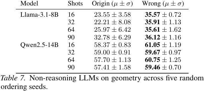
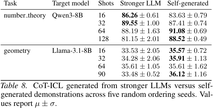
At a 32-shot setting, LLaMA 3.1 (8B) reaches only 22.21% accuracy with reference answers (origin), but jumps to 35.91% using its own wrong answers. Feeding it examples generated by a stronger model (e.g. Qwen 2.5 14B) also performs markedly worse (33.53%–34.28%) than feeding it its own self-generated examples (35.57%–35.91%).

6.3 CDS Ordering Delivers Stable, Cross-Model Gains

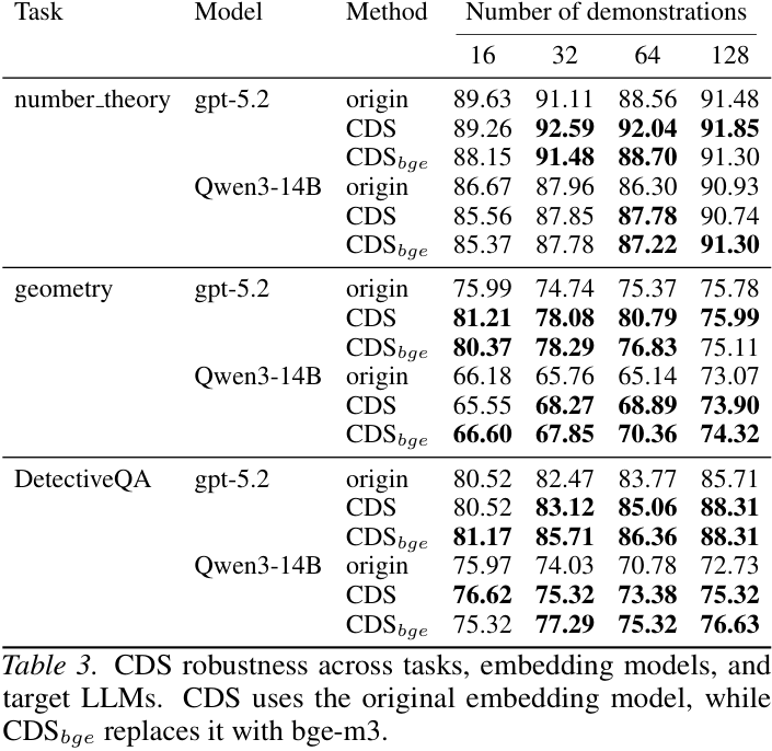
On Qwen3-14B’s geometry task (64-shot), random ordering reaches only 65.14% accuracy, while CDS ordering raises it to 68.89%; swapping in the open-source bge-m3 embedding for ordering pushes it further to 70.36%. This gain isn’t a single-model coincidence — with the closed-source gpt-5.2 on number theory (32-shot), CDS likewise lifts accuracy from 91.11% under random ordering to 92.59%, showing the method is picky about neither the embedding model nor the LLM.

6.4 Curvature Is the Causal Variable, Not Just a Clustering Effect

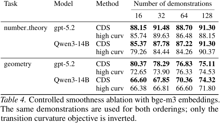
To rule out the objection that “CDS only works because it groups similar problems into the same block,” the authors designed a control condition that deliberately manufactures hairpin turns (high curv) — both conditions use Euclidean distance to cluster similar problems together, but the high-curv condition deliberately picks the sharpest-turning arrangement at block transitions. Both comparisons come out decisively: on number theory (16-shot), Qwen3-14B scores 85.37% with CDS versus only 79.26% with high curv; on geometry (16-shot), gpt-5.2 scores 80.37% with CDS but drops to 72.65% with high curv — a gap of 7.72 percentage points. This shows the turning angle is itself a causal factor behind the performance difference, not a byproduct of clustering.

7 Conclusion

The paper’s core conclusion can be compressed into two lines for prompt engineering practitioners: content should be understandable, ordering should flow. When picking example content, rather than chasing perfect solutions generated by the strongest available model, prefer chains of thought generated by the target model itself — even with the occasional flaw, the absorption benefit from distributional alignment comes out ahead. When ordering examples, rather than relying on traditional RAG retrieval by semantic similarity, use something like CDS to minimize curvature and lay out a reasoning path with no hairpin turns for the model.

CDS itself is computationally cheap and touches no model parameters, making it a good fit to drop straight into an existing LLM pipeline as a prompt-preprocessing layer — this “don’t change the model, just change the prompt” route is the same class of engineering leverage as zero-latency preprocessing tricks like Prompt Repetition. Looking ahead, one natural extension is combining it with existing RAG architectures, so retrieval-augmented generation selects not just “knowledge fragments” but also a well-ordered “reasoning trajectory”; another direction worth watching is whether this mechanism of “a model reading its own generated reasoning traces to improve itself” has room to work in multi-step decision tasks like agent planning or code generation.