Better & Faster Large Language Models via Multi-token Prediction

1 Introduction
On June 18, 2024, Meta AI announced the release of several new AI models on the Meta Blog. Among them, one particularly interesting model is the “Multi-Token Prediction Model.”
Meta has long been a key contributor to the AI open-source community, and as expected, the pre-trained models are available on HuggingFace. In fact, the paper describing this model was uploaded to Arxiv back in April of this year. However, it didn’t seem to garner much attention until Meta’s official announcement and open-source release.
In this article, I aim to provide a simple and quick overview of the paper’s content, covering the problem it addresses, the design of its solution, and the final experimental results.
2 The Motivation Behind Multi-Token Prediction
Nearly all Large Language Models (LLMs) we see today—about 99% of them—are Auto-Regressive Models. This means that during both training and inference, these models perform the task of Next-Token Prediction: predicting the (t+1)-th token based on the sequence of tokens from 1 to t.
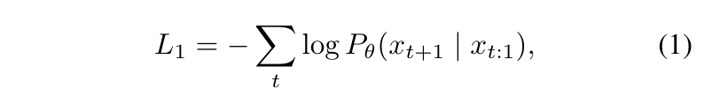
During the training phase, the loss function typically looks like Equation (1) below:
The problem this paper addresses is quite intuitive: Why must we predict only one token at a time? Why not predict multiple tokens at once?
3 The Design of the Multi-Token Prediction Model
To predict multiple tokens at once, the loss function used during training must be modified, as shown in Equation (2):

The key difference is that instead of calculating a single Cross-Entropy Loss from the probability distribution of one predicted token, we now calculate ’n’ Cross-Entropy Losses from the probability distributions of ’n’ predicted tokens. These ’n’ losses are then summed up to update the model.
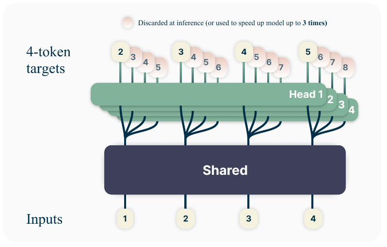
Beyond the loss function, the model’s architecture (shown above) primarily uses a Shared Transformer Trunk (which you can think of as a single, shared encoder) to generate a hidden representation that encodes the information of the preceding t tokens. This representation is then fed into ’n’ separate heads, each predicting one of the next ’n’ tokens.
We can see the architecture is quite straightforward. However, a practical issue arises during training: in an LLM’s forward pass, the dimensionality of the final logits is much larger than that of the intermediate hidden representations. Therefore, if we were to compute all ’n’ tokens in parallel for multi-token prediction, the GPU memory required for the logits would increase ’n’-fold. To mitigate this high GPU memory usage, the paper proposes a sequential approach for predicting each token:
As shown on the left side of the diagram above, after obtaining the hidden representation from the Shared Transformer Trunk based on an input sequence:
- The representation is first fed into Head #1 to get the #1 predicted token and its loss. A backward pass is performed on this loss to accumulate gradients in the hidden representation.
- It is then fed into Head #2 to get the #2 predicted token and loss, and another backward pass accumulates more gradients in the hidden representation.
- This process continues for all N tokens.
- Finally, another backward pass is performed on the accumulated gradients in the hidden representation to calculate the gradients for the weights in the Shared Transformer Trunk.
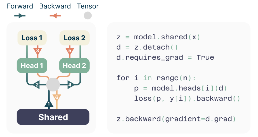
The pseudocode on the right clearly illustrates this. After the input sequence (x) passes through the Shared Transformer Trunk to get the hidden representation (z), the detach() method is called to create a new tensor, d.
Tensor d has the same values as tensor z, but the detach() method removes it from the computation graph of z. The effect of this is that when we call backward() on any tensor derived from d, the gradient calculation will only go as far back as d itself, not further back to z, model.shared, or the input x.
Specifically, in the for loop in the lower half of the pseudocode, tensor d undergoes some operations to produce tensor p (the prediction from one of the heads). Then, a loss is calculated using p and the label, and backward() is called. This is the crucial step. At this point, gradients are only computed for “tensor p,” the weights/biases in model.heads[i], and tensor d.
Why don’t the gradients flow back to z and model.shared?
Because the detach() method has removed d from their computation graph! Additionally, since the tensor d is identical in each iteration of the for loop, the gradients calculated from each head’s loss are stored in d.grad. By default, PyTorch accumulates gradients, which means all gradients for d are summed up. Only after the loop finishes is z.backward(gradient=d.grad) manually called, using the accumulated gradients in d.grad to compute the gradients for z (and subsequently, the weights of model.shared).
You can see that this sequential processing of each head is designed to avoid:
- Simultaneously materializing all head logits during the forward pass.
- Simultaneously calculating gradients for the entire model from all head losses during the backward pass.
This, in turn, reduces peak GPU memory usage.
During inference, this architecture offers flexibility. You can use only the first prediction head for standard next-token prediction, or retain all heads to implement techniques similar to Speculative Decoding.
4 Experimental Results of the Multi-Token Prediction Model
Now that we understand the design of the Multi-Token Prediction Model, let’s look at the experiments. To save you time, here is a summary of the results.
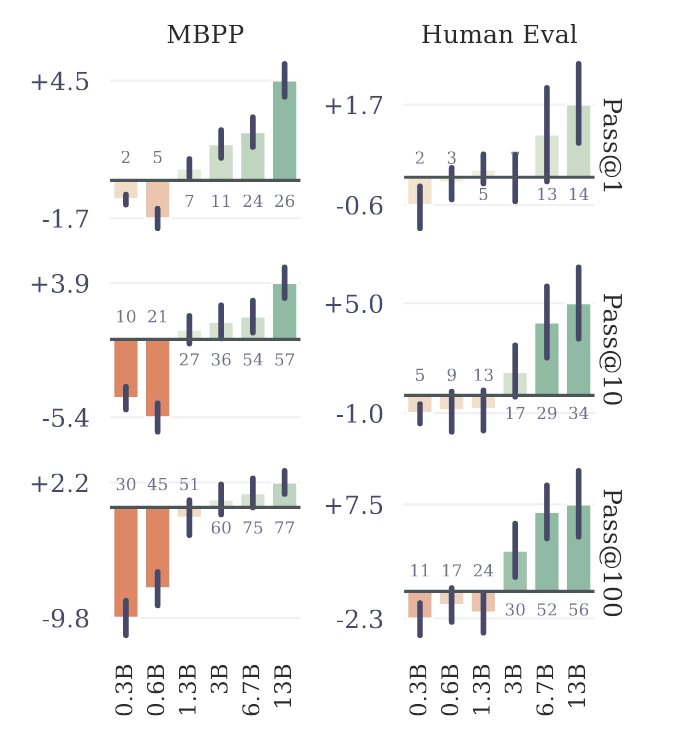
First, the graph above shows that when evaluating six different model sizes on two benchmarks (MBPP and HumanEval), multi-token prediction actually performs worse on smaller models. However, for larger models, it generally yields better results. The authors speculate this might be why multi-token prediction methods have not been popular in the past.

The authors found that when training a 7B byte-level Transformer (one that predicts the next byte instead of the next token), the multi-byte prediction pre-training task significantly outperforms the next-byte prediction pre-training task (as shown in the first row of the table above).
Furthermore, the second row of the table shows that for token-level transformers, 4 prediction heads usually yield the best results. In contrast, for byte-level transformers (first row), 8 prediction heads are more effective. This suggests that the optimal number of prediction heads is related to the input data distribution. Nevertheless, multi-token (or multi-byte) prediction generally proves superior to its single-token (or single-byte) counterpart.
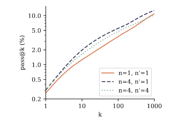
In the graph above, the authors pre-trained a 7B model in two ways: with Next-Token Prediction (solid orange line, n=1) and 4-Token Prediction (black and green dashed lines, n=4), and then fine-tuned the models. During fine-tuning, they used either next-token (n’=1) or 4-token (n’=4) prediction. As you can see, regardless of the value of k, the models pre-trained with 4-token prediction (black and green dashed lines) outperform the baseline pre-trained with next-token prediction (solid orange line). This demonstrates the effectiveness of using a multi-token task during the pre-training phase.
5 Conclusion
In this article, we’ve explored Meta’s recently published and open-sourced Multi-Token Prediction Model. Unlike the vast majority of current LLMs, which are trained using next-token prediction, Meta discovered that for LLMs larger than 3 billion parameters, training with a multi-token prediction task can actually enhance model performance. We also delved into the model’s architecture and its clever use of sequential prediction to reduce GPU memory consumption.