Your Base Model Is Smarter Than You Think: How MCMC Sampling Can Outperform RL

1 Introduction

In this article, I’d like to share the paper Reasoning with Sampling: Your Base Model is Smarter Than You Think. This paper was uploaded to arXiv in October 2025 and has been submitted to the ICLR 2026 Conference. While the final acceptance results are not out yet, judging by the Reviewers’ scores, it promises to be an excellent paper!

The main reason I wanted to read this paper is that it challenges the current mainstream view (Reinforcement Learning (RL) for Reasoning). It proposes that by using Sampling methods during the Inference stage, a Base Model can achieve or even surpass the reasoning capabilities of an RL Model.

2 The Problem This Paper Aims to Solve

To understand the problem this paper attempts to solve, we need to (1) understand the concept of Distribution Sharpening and (2) understand the paper’s hypothesis regarding RL.

2.1 What is Distribution Sharpening?

Distribution Sharpening is an operation performed on a probability distribution.

Imagine we have a Base Model predicting the next Token or generating a complete reasoning path. It possesses a probability distribution $p(x)$.

• Some answers have a very high probability (e.g., logical reasoning).
• Some answers have a very low probability (e.g., gibberish).
• Many answers lie somewhere in between.

Sharpening is the process of using mathematical operations to make the parts with originally high probability even higher, and the parts with low probability even lower.

Represented by a mathematical formula, if we have a parameter $\alpha > 1$, the relationship between the sharpened probability $p_{sharp}(x)$ and the original probability is:

Using a real-life analogy, this is like adjusting the “contrast” in photo editing software: making grey areas black and light grey areas white. In the world of models, it forces the model to “believe more strongly” in the answers it already thought were relatively good (by increasing their probability), while suppressing the answers it felt were poor (by decreasing their probability).

2.2 The Paper’s Hypothesis on RL

This paper mentions Distribution Sharpening to reinterpret the impact of RL on a model’s reasoning capabilities. This is the theoretical foundation of the entire paper!

Currently, powerful reasoning models like OpenAI o1 or DeepSeek-R1 are achieved through Post-training using RL (e.g., PPO, GRPO). However, there is a huge debate in the academic community: Does RL actually teach the model “new” reasoning capabilities?

• Viewpoint A: RL teaches the model logic it didn’t know before.
• Viewpoint B (Supported by this paper): RL does not teach the model new things. It merely “excavates” the correct reasoning paths that are already implicit and existing within the Base Model, and “sharpens” the probability of these paths through training.

Therefore, the authors believe that the behavior exhibited by a model trained with RL is actually equivalent to a “Sharpened Base Model”. In other words, the Base Model already knows the correct answer (Smarter Than You Think), but these correct reasoning paths are drowned out by a vast number of mediocre paths, making their probabilities insufficiently prominent. RL training is equivalent to sharpening the Base Model, making the probability of correct reasoning paths higher and incorrect ones lower.

Returning to the problem this paper wants to solve:

If the essence of RL is merely Distribution Sharpening, why spend a fortune on training? Can we simulate this sharpened probability distribution directly using algorithms at Inference Time?

3 The Method Proposed in This Paper

Summarized in one sentence:

Sampling from the Base Model’s Sharpened Distribution using Markov Chain Monte Carlo methods.

To solve the aforementioned problem, the paper proposes Distribution Sharpening and an Inference-Time Sampling method. The authors don’t want to directly train the Base Model into an RL Model. Instead, they take the Base Model’s original probability distribution $p(x)$, sharpen it to become $p(x)^\alpha$, and then sample from this Sharpened Distribution to achieve output performance comparable to an RL Model.

Note that $p(x)$ here refers to the probability of the Base Model generating a complete reasoning path (i.e., Joint Probability), not the probability of generating a single Token. This distinguishes “Sampling from a Sharpened Distribution” from the commonly seen “Low-temperature Sampling”!

3.1 Why Use Markov Chain Monte Carlo?

So far, we understand the author’s goal is to sample from the sharpened distribution $p(x)^\alpha$, where $p(x)^\alpha$ refers to the probability of the entire reasoning path, not a single Token.

Here comes the problem. Assuming the vocabulary size is $V$ and the length of the generated reasoning path is $T$, the total number of possible reasoning paths is $V^T$. This is an astronomical number.

To sample directly from a probability distribution, we usually need to know the Normalized Probability of every possible path:

Here $Z$ (Normalization Constant) is the sum of probabilities of all possible reasoning paths:

The issue is we cannot calculate $Z$ because there are $V^T$ paths. However, we can easily calculate the numerator $p(x)^\alpha$. This is because $p(x)$ is the Likelihood of the reasoning path by the Base Model, which is the Joint Probability calculated in a single Forward Pass.

This is exactly why Markov Chain Monte Carlo is needed. The most powerful aspect of MCMC algorithms is: It doesn’t need to know $Z$; it only needs to know the “relative strength between two samples” to sample from the target distribution. In other words, with MCMC, we don’t need to calculate the probabilities of all possible paths, sharpen them, and then sample. As long as we can calculate $\frac{p(x_{new})^\alpha}{p(x_{old})^\alpha}$ for any two reasoning paths, MCMC works.

3.2 What is Markov Chain Monte Carlo?

Markov Chain Monte Carlo can be literally broken down into two parts:

• Monte Carlo: Refers to methods solving problems via “random sampling”.
• Markov Chain: We design a state machine that jumps between different states (here, different reasoning paths).

Core Idea: We don’t want to generate a perfect reasoning path out of thin air (too hard). We want to construct a Markov Chain such that when this Chain runs long enough, the frequency with which it stays in a certain state (reasoning path) equals our desired target probability $p(x)^\alpha$.

This is like designing a robot to randomly wander in a space filled with reasoning paths. We set rules for it:

• If it walks to a “good reasoning path (high probability)” area, stay there a bit longer.
• If it walks to a “bad reasoning path (low probability)” area, leave quickly or don’t go there at all.

Eventually, we record all the states the robot visited. These states are the samples drawn from the $p(x)^\alpha$ distribution.

3.3 The Classic MCMC Algorithm - Metropolis-Hastings

This paper specifically uses the most classic algorithm in the MCMC family: Metropolis-Hastings.

Its workflow is very intuitive, divided into three steps:

Step 1: Current State

Assume we already have a generated reasoning path, let’s call it $x$ (e.g., an ordinary problem-solving process).

Step 2: Proposal

We need a mechanism to “randomly modify” this path to produce a candidate new sentence $x'$. Therefore, we randomly select a position $t$, chop off all words after $t$, and let the Base Model Resample the second half. This “regeneration” process is called the Proposal Distribution $q(x'|x)$.

Step 3: Accept or Reject

This is the most critical step! We must decide: jump to the new sentence $x'$, or stay with the old sentence $x$? Thus, we calculate an Acceptance Ratio $A$:

Let’s look at its physical meaning:

1. Likelihood Ratio ($\frac{p(x')^\alpha}{p(x)^\alpha}$):

   • If the score of the new path $x'$ is higher than the old one $x$, this value is greater than 1.

2. Proposal Correction ($\frac{q(x|x')}{q(x'|x)}$):

   • This is to correct the bias of the Proposal action itself (if symmetric, this term is usually 1).

Rules:

• After calculating $A$, we generate a random number $u$ between 0 and 1.
• If $u < A$, we Accept the new sentence, and the state becomes $x'$.
• Otherwise, we Reject it, and the state remains at $x$ (i.e., try again).

3.3.1 How many Tokens to cut? How to set $t$?

Theoretically, we could cut the last $t$ Tokens. However, the algorithm proposed in the paper (Algorithm 1) is a bit more refined; it operates in Blocks.

• Sequential Block Generation:

  The author doesn’t generate a full Trace of hundreds of Tokens and then start MCMC. They slice the length $T$ into many small blocks, each of length $B$ (e.g., $B=192$ tokens).

  1. First generate the first Block.
  2. Perform MCMC optimization on this “First Block” (repeatedly cut and regenerate).
  3. Once satisfied (or iterations done), Fix this Block.
  4. Then generate the second Block… and so on.

• How to cut within a Block?

  When performing MCMC on the current Block, it randomly selects a cut point $m$.

  • For example, if the current Block has 192 Tokens.
  • In this iteration, it might randomly pick the 50th Token, chop everything after 50, and recalculate.
  • The next iteration might pick the 180th token, recalculating only a tiny bit at the end.

  Therefore, $t$ is not fixed; it is a cut point randomly selected within the current Block range.

3.3.2 How many times to repeat? When to stop?

Theoretical MCMC needs to run infinitely to converge perfectly, but in engineering, we have a Compute Budget.

• Parameter Setting: The paper has a parameter called $N_{MCMC}$.
• Workflow: For every Block (e.g., 192 Tokens), we forcibly run the “Regenerate -> Compare” cycle $N_{MCMC}$ times.
• Stop Condition: After running $N_{MCMC}$ times (e.g., 10 or 20 times), we assume the Trace we have now is good enough, fix it, and move to the next Block.
  • It stops when “time is up”, not when “a certain probability is reached”.

3.3.3 What guarantees MCMC finds the correct Trace? What if the Proposal is worse?

The guarantee of MCMC comes from the game between the “Accept/Reject Mechanism” and “Randomness”.

• Case A: The Proposed Trace has a higher probability (Better quality path)

  • According to the formula, Acceptance Ratio $A > 1$.
  • We 100% Accept this new one. It’s like climbing a mountain; if you see a higher spot, you climb up.
  • Result: The Trace in our hand gets stronger.

• Case B: The Proposed Trace has a lower probability (Worse quality path)

  • This is common, as random changes usually break things.
  • According to the formula, Acceptance Ratio $A < 1$ (e.g., $A=0.1$).
  • We have a $10\%$ chance to accept it, and a $90\%$ chance to Reject it.
  • Key Point: If rejected, we revert to the previous better state, not stay in the bad state. So the Trace in our hand stays the same at worst.

• Why does it converge? Although the Proposal often gives bad results, as long as the Base Model has a non-zero probability of generating that “Good Trace”, after enough attempts, it will eventually “stumble upon” a better fragment. Once it stumbles upon it (Case A), we accept and lock it as the new Baseline. The next attempt must find something even better to update. This is like a random trial with an insurance mechanism: keep it if improved, revert if worsened (mostly).

3.3.4 Why use Sharpening parameter $\alpha$ in Acceptance Ratio $A$?

In calculating Acceptance Ratio $A$:

• If $\alpha = 1$ (No Sharpening):

  If the new sentence is 2x more likely than the old, acceptance is 2 (Accept). If the new sentence is 0.5x as likely, acceptance is 0.5.

• If $\alpha = 4$ (High Sharpening, common in paper):

  If the new sentence is 2x more likely, acceptance becomes $2^4 = 16$ (Super Accept). If the new sentence is 0.5x as likely, acceptance becomes $0.5^4 = 0.0625$.

Conclusion: $\alpha$ determines our sensitivity to “quality”. The larger $\alpha$ is, the more “snobbish” the algorithm becomes: craving high-scoring sentences intensely, and rejecting low-scoring ones extremely. This is the driving force forcing the model to converge towards high-probability regions (correct reasoning).

3.3.5 Why not just “always” choose the higher probability path in (Step 3)? Why calculate an acceptance rate?

This is the fundamental difference between Optimization and Sampling. If our goal is purely to pick the biggest, it’s called Hill Climbing, and in that case, we wouldn’t even need $\alpha$ or acceptance calculations, just if new > old then accept.

But this paper uses MCMC and must include $\alpha$ for two reasons that “just picking the biggest” cannot replace:

1. To Escape Local Optima

   If you adopt the “Deterministic (Only pick bigger)” strategy:

   • Scenario: You are at the top of a small hill (Reasoning Trace is okay, but not best).
   • Problem: Any modification (Proposal) causes a temporary probability drop (stepping down the hill).
   • Result: Because your rule is “only pick bigger,” you will forever reject these changes. You are trapped on this small hill, never reaching the higher Mount Everest (Correct Answer) next door.

   The Wisdom of MCMC: It allows you to occasionally accept worse results (Probabilistic Acceptance).

   • This is like allowing yourself to walk “downhill” for a bit while hiking, giving you the chance to cross the valley and climb the higher mountain opposite.

   Role of $\alpha$: Without $\alpha$ (e.g., $\alpha=1$), MCMC accepts bad results too easily (goes downhill too much), wasting time on wrong paths. With $\alpha$ (e.g., $\alpha=4$), we widen the probability gap.

   • For “slightly worse” paths: Acceptance rate lowers slightly, chance to jump remains.
   • For “much worse” paths: Acceptance rate crashes exponentially, almost impossible to accept.

   So, $\alpha$ is the parameter controlling how much risk we are willing to take to Explore.

2. Mathematical Necessity

   This returns to the paper title: Distribution Sharpening. Our target distribution to simulate is not the Base Model’s original $p(x)$, but the sharpened $p(x)^\alpha$.

   According to Metropolis-Hastings derivation, the Acceptance Ratio $A$ must equal the “Ratio of Target Probabilities”.

   $$A = \frac{\text{Target}(x_{new})}{\text{Target}(x_{old})}$$
   • If target is $p(x)$, ratio is $\frac{p(x_{new})}{p(x_{old})}$
   • But our target is $p(x)^\alpha$, so ratio must be: $\frac{p(x_{new})^\alpha}{p(x_{old})^\alpha} = \left( \frac{p(x_{new})}{p(x_{old})} \right)^\alpha$

   Physical Meaning: $\alpha$ acts like a “magnifying glass” or “contrast knob”.

   Suppose $x_{new}$ is slightly better than $x_{old}$, probability is $1.2$x.

   • No $\alpha$: Acceptance 1.2. Advantage 20%.
   • With $\alpha=4$: Acceptance $1.2^4 \approx 2.07$. Advantage becomes 107%.

   Suppose $x_{new}$ is slightly worse, probability is $0.8$x.

   • No $\alpha$: Acceptance 0.8. You have 80% chance to accept this worse result (too easily swayed).
   • With $\alpha=4$: Acceptance $0.8^4 \approx 0.41$. You only have 41% chance to accept it.

Summary: You need $\alpha$ because:

1. Algorithm Behavior: $\alpha$ makes the algorithm more sensitive to quality. It forces the model to be “greedier, but not rigid”.
2. Math Definition: Your target is the Sharp Distribution; the formula dictates the ratio takes the power.

3.3.6 What is Proposal Correction in Metropolis-Hastings?

Simply put, this term exists for “Fairness”.

Let’s look at this part of the formula:

• Denominator (Forward): How easy is it to jump from $x_{old}$ to $x_{new}$?
• Numerator (Backward): If we are at $x_{new}$, how easy is it to jump back to $x_{old}$?

1. Why do we need this correction? (Intuitive Explanation)

   Imagine a game where we randomly visit rooms (reasoning paths). Our goal is to visit “beautiful rooms” (high probability paths).

   However, our movement method (Proposal) is biased:

   • Some rooms have 10 entrances; it’s easy to walk in accidentally.
   • Some rooms have only 1 entrance; hard to find.

   If we don’t correct this bias, we will mistakenly think those “many-entrance” rooms are more beautiful, causing us to stay there too long.

   Proposal Correction eliminates the bias caused by “number of entrances”.

   • If a new path $x_{new}$ is very easy to generate (large denominator), it means the Proposal is biased towards it. To be fair, we deduct points (divide by a large number) in the formula.
   • Conversely, if a new path is rarely generated, we add points.

   This ensures that whether we stay in a room depends only on whether the room is beautiful ($p^\alpha$), not on how easy the door is to enter.

2. What does this mean in this paper? (Math Derivation)

   In this paper’s algorithm, this term has a special mathematical effect.

   • Proposal ($q$): The authors use the Base Model directly to generate new segments. So the probability of generating a new suffix is simply the Base Model’s original probability $p(suffix)$.

   Let’s plug this into the formula (Assuming Prefix is fixed for simplicity):

   1. Target Ratio: The ratio we want.

      $$\frac{p(x_{new})^\alpha}{p(x_{old})^\alpha}$$

   2. Correction Term:

      • Prob from Old to New $\propto p(x_{new})$ (Generated by Base Model)
      • Prob from New to Old $\propto p(x_{old})$
      • So correction term is: $\frac{p(x_{old})}{p(x_{new})}$

   3. Final Acceptance Ratio:

      $$A = \underbrace{\left( \frac{p(x_{new})}{p(x_{old})} \right)^\alpha}_{\text{What we want}} \times \underbrace{\left( \frac{p(x_{old})}{p(x_{new})} \right)}_{\text{Correction Term}}$$

      Merging via exponent rules:

      $$A = \left( \frac{p(x_{new})}{p(x_{old})} \right)^{\alpha - 1}$$

   From this result, we see that without the correction term, we tend to accept sentences the Base Model thinks are high probability (because the Proposal keeps pushing them). With the correction, we cancel out the Base Model’s original Bias once (minus 1).

4 Experimental Results of the Paper

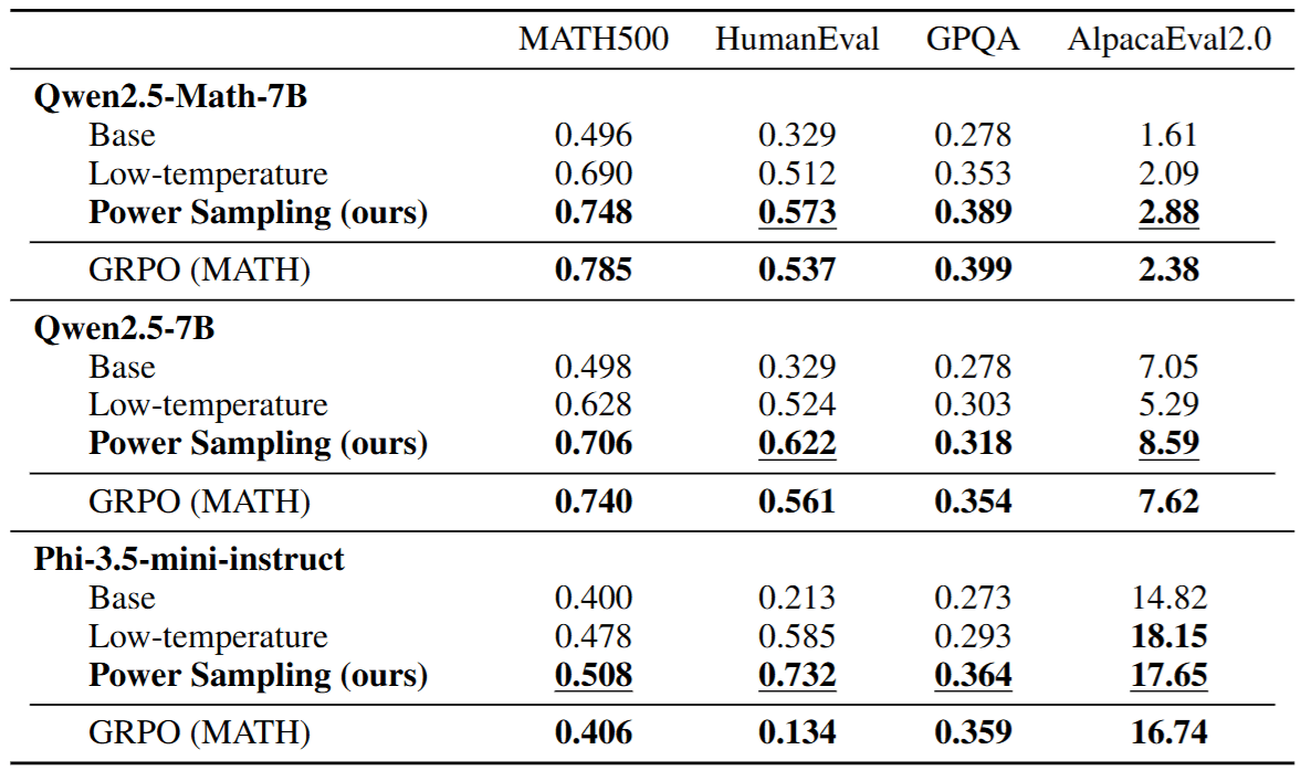
Finally, here are the main experimental results. We can see that simply performing Sampling on the Base Model indeed achieves or surpasses the performance of RL (e.g., GRPO) Models on many Benchmarks.

5 Conclusion

In this article, I shared the paper Reasoning with Sampling: Your Base Model is Smarter Than You Think. Whether reading the paper or writing this post, I felt incredibly enlightened!

What I find most interesting is not just that it proposes a sampling algorithm based on Markov Chain Monte Carlo, but that it offers a philosophical reflection on the current path of AI development: Have we underestimated the potential of the Base Model and overly mythologized the role of RL?

Reviewing the entire article, we can summarize three points worth pondering:

5.1 The Essence of Reasoning: “Learning” or “Searching”?

In the past, we tended to think models needed RL (e.g., PPO, GRPO) to “learn” logical reasoning. But through the lens of Distribution Sharpening, this paper tells us that perhaps the essence of reasoning is more like a process of extracting signal from noise.

The Base Model is like a student who has read ten thousand books but lacks confidence. The correct answer is actually in their mind (Latent Space), just drowned out by a mass of mediocre responses. We don’t need to reteach them knowledge via RL; we just need to give them a little time and guidance (Sharpening & Sampling) to let them deliberate repeatedly, and the correct reasoning path will naturally emerge. This is the true meaning of the title “Your Base Model is Smarter Than You Think”.

5.2 The Rise of Inference-time Compute (System 2 Thinking)

The method in this paper is a perfect embodiment of the Inference-time Compute trend.

• System 1 (Fast Thinking): Direct output of the Base Model, relying on intuition, fast but prone to errors.
• System 2 (Slow Thinking): The MCMC Sampling proposed here, relying on repeated deliberation, backtracking, and correction, slow but logically rigorous.

Although Markov Chain Monte Carlo requires more Inference time and compute than usual (due to constant Proposing and Rejecting), this implies we can “Trade Time for Intelligence”. Unlocking powerful reasoning capabilities merely by changing the sampling strategy, without retraining massive models, is undoubtedly an attractive path for researchers or enterprises with limited resources.

5.3 Future Outlook: The Dance of RL and Sampling

Of course, this doesn’t mean RL will be eliminated (impossible, haha). The authors also mention that if a Base Model is completely ignorant about a field (probability is 0), then even the strongest Sharpening is futile.

Perhaps the future trend will move towards a hybrid mode: using RL for lightweight alignment to ensure the general direction of the Base Model’s probability distribution is correct; then, during the Inference stage, dynamically introducing strategies like the Markov Chain Monte Carlo proposed in this paper for deep searching on high-difficulty reasoning problems.

In conclusion, this is an interesting and fantastic paper. I hope this article brings you value!