RAGU: The Paper That Accidentally Measured GraphRAG's Ceiling

1 Introduction
RAGU is a GraphRAG engine that a team from ITMO University put on arXiv in July 2026, shipped alongside a 7B extraction model called Meno-Lite-0.1. Both are open source (pip install graph_ragu, MIT licensed). The paper’s claim is that splitting knowledge-graph “extraction” and “consolidation” into two separate stages yields a cleaner graph and more complete retrieval.
This article is not just about what RAGU does, but about what is left once you take its experimental design apart. The conclusion is a little counterintuitive: the paper’s own research contribution is thin, but buried in its data tables is a number very few people are willing to publish — the net contribution of the entire GraphRAG stack, relative to building no graph at all and doing pure vector retrieval, is only 1.2 to 4.3 percentage points. That number is worth more than anything the paper set out to prove.
Along the way we will pick up three ideas that hold well beyond this particular paper: why deduplication and clustering are two different tasks, how “similarity” differs between graph clustering and vector clustering, and — most importantly — why good retrieval metrics do not mean good answers.
2 What problem is GraphRAG solving?
Some background first. Standard RAG cuts documents into chunks, turns them into vectors, and at query time pulls back the few most similar chunks to stuff into the prompt. This retrieval is flat: every chunk stands alone, and the system cannot see relationships that span documents. If the answer depends on the link between “a person mentioned in document A” and “a company mentioned in document B,” vector similarity will not find it. (Chunking strategy is a discipline of its own — see the discussion in Adaptive Chunking.)
GraphRAG’s answer is to first have an LLM extract the entities (people, organizations, products) and relations in the documents and build them into a knowledge graph, so retrieval can walk along the graph’s edges. The representative systems on this path are Microsoft GraphRAG, LightRAG, and HippoRAG 2. (There is also a movement in the opposite direction — SAG, for instance, argues for skipping the offline knowledge graph entirely and joining events with SQL at query time.)
RAGU identifies three problems with existing systems: they extract once and build the graph immediately, producing a mass of duplicate and noisy entities with no mechanism for cross-chunk consolidation; they assume a GPT-4-class model for extraction, which is too expensive; and the engineering quality of open-source frameworks varies wildly, to the point of unsafe paths like running eval() directly on raw LLM output. RAGU addresses these three with, respectively, a multi-step pipeline, the 7B Meno-Lite-0.1, and a seriously written engineering implementation.
3 The “7B is enough” hypothesis, and what’s wrong with it
The paper’s core scientific claim is that what an LLM does inside a RAG pipeline — understanding context, extracting entities, summarizing, generating answers from context — is a language skill, not world knowledge. Language skills scale very slowly with model size; world knowledge scales fast. Therefore 7B is enough on the extraction side.
The evidence is this figure:
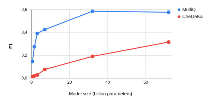
The two tasks differ in nature: CheGeKa is a Russian-language general-knowledge quiz with no context, testing purely memorized knowledge; MultiQ is multi-hop QA where all the facts are in the context. The numbers the paper reports, from 0.5B to 72B, are 21.1× growth for CheGeKa and only 4× for MultiQ.
That comparison is inflated. CheGeKa’s F1 at 0.5B is essentially on the floor (about 0.015), so the denominator approaches zero and any growth converts into a dramatic multiple. MultiQ starts high (about 0.12) and hits its ceiling somewhere around 32B (flat after roughly 0.57), so part of its small multiple is simply saturation. What actually holds up is the log-linear slope in the same figure, 0.65 versus 0.26 — at least that is a comparison on a single scale. Yet the paper put “21.1× vs. 4×” in the abstract as the headline.
There are two further problems. First, MultiQ measures “read the context and answer the question,” but the pipeline’s truly critical action is extracting structured entities and relations — and the paper’s own information-extraction experiment shows the plain Qwen2.5 family improving monotonically with scale on extraction (7B 0.356 → 14B 0.396 → 32B 0.416). Second, both benchmarks are Russian, and CheGeKa in particular is Russian cultural trivia; using it to stand for “world knowledge” and then generalizing to an English medical corpus is not a small leap.
3.1 The claim it should have made: the task sits in the saturated region
“Language skills don’t scale with model size” contradicts reality. Today’s SOTA models are precisely a demonstration of scaling laws, with reasoning ability improving steadily with model and data scale. The more accurate statement would be:
The tasks in this pipeline are easy enough to fall in the saturated region of scaling.
The difference is the ceiling effect. A task like “pull the person’s name out of this sentence” has its difficulty distribution concentrated in the easy region: 7B might already score 85 and 72B only 90, so there was never room for scale to show. Tasks like AIME (competition math) or GPQA (graduate-level science QA), with their multi-step derivations, have a hard tail — 7B scores 5, a large model scores 80, and the effect of scale is plain to see.
The practical takeaway is the same either way: for pipeline components whose job is “understand and move information around,” a small model is usually enough. But the reason is “the task is easy,” not “scale doesn’t work.” Get the reason wrong and you will misapply it to the parts that genuinely need reasoning.
Incidentally, the paper’s evidence comes from Qwen2.5-Instruct, a 2024 non-reasoning family. The main gains in modern reasoning models come from the RL post-training axis, which the paper does not touch at all.
3.2 Why the paper needs this hypothesis
This deserves its own section, because it is useful when reading other system papers: without this hypothesis, Meno-Lite-0.1 is not a research contribution, just a cost saving.
Without the hypothesis → "we trained a small model because we can't afford a big one"  = engineering compromise
With the hypothesis    → "we found big models are wasteful; small ones suffice in principle" = key insight
The line in the abstract — “A key insight motivates a compact extractor” — is doing exactly this: supplying a post-hoc theoretical justification for a decision that was already made. It simultaneously props up the cost narrative ($0.001/doc vs. $0.10/doc, which is only persuasive if “small models don’t sacrifice quality” holds), and it later provides an angle for rewriting bad news as good when Meno-Lite-0.1’s advantage disappears.
4 Method: six steps, one of them original
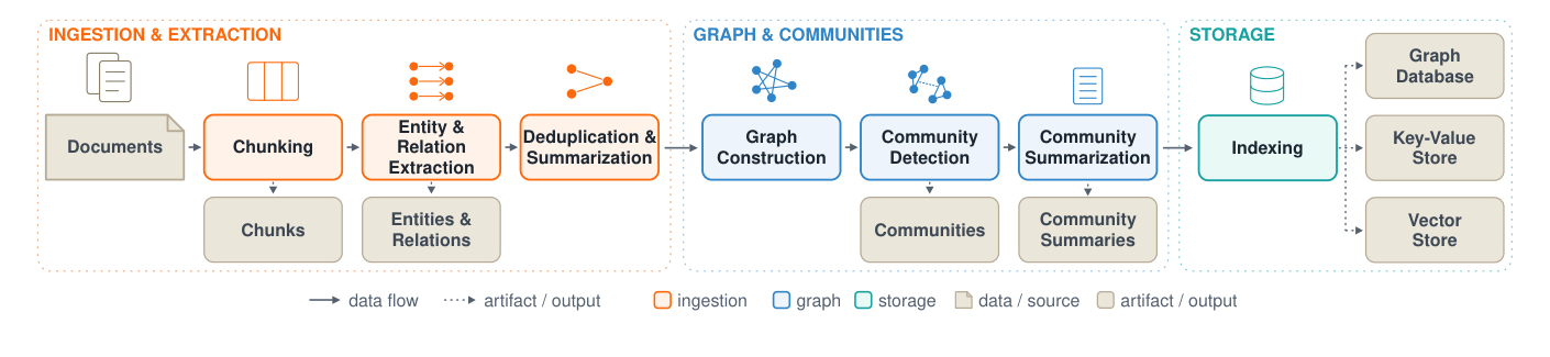
The flow itself is easy to follow:
Documents
   ↓  Step 1  Chunking
Chunks
   ↓  Step 2  Entity & Relation Extraction   ← two-stage, schema-constrained
Entities & Relations (very dirty: duplicates, aliases, noise)
   ↓  Step 3  Deduplication & Summarization  ★ the paper's only original cell
Entities & Relations (clean)
   ↓  Step 4  Graph Construction
   ↓  Step 5  Community Detection (Leiden)
   ↓  Step 6  Community Summarization
Compared with Microsoft GraphRAG and LightRAG, the only difference is Step 3; every other cell is an existing technique.
“Clean before you build the graph” makes sense in principle. Community detection clusters based on the graph’s connection structure, so if one entity gets split into three nodes (“Dennis Ritchie” / “Ritchie” / “D. Ritchie”), the 3 edges that should have been concentrated get scattered as 1+1+1, that node becomes structurally unimportant, and it may be assigned to the wrong community or end up isolated. In other words, noise in the extraction stage gets amplified by community detection into a structural error — one that nothing downstream can fix.
4.1 Step 2: two-stage extraction turns generation into multiple choice
Extraction is split into two LLM calls:
Stage 1: chunk → extract entities → validate types against the NEREL schema
         produces a validated entity set E = {e1, e2, ...}

Stage 2: chunk + E → extract relations
         constraint: every relation's source_entity and target_entity
                     must be a name already validated in E
What this fixes is dangling edges. In single-pass extraction, an LLM often writes names into relations that do not exist in the entity list — it extracts the entity “Bell Laboratories” but writes “Bell Labs” in the relation, and the edge now points at a node that does not exist. The two-stage approach pins down “which nodes exist” first, so the second stage goes from open-ended generation to multiple choice over a closed set.
This pattern generalizes beyond GraphRAG: any time you want an LLM to produce output that refers to existing things, fix the legal options first and then let it choose. It is the same line of thinking as constrained decoding.
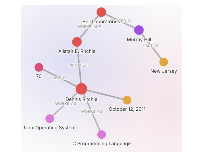
As for how the types are defined, the NEREL schema the paper uses has 29 entity types and 49 relation types, drawn from an annotation scheme for a Russian news corpus. The paper itself concedes in its Bias section that changing language or domain may require redesigning the schema — and its own hand-picked demo gives the game away. The Dennis Ritchie passage yields 8 relations, of which the paper shows 5:
| Source | Target | Relation |
|---|---|---|
| Dennis Ritchie | C Programming Language | WORKS_AS |
| Dennis Ritchie | Unix Operating System | WORKS_AS |
| Dennis Ritchie | October 12, 2011 | DATE_OF_DEATH |
| Alistair E. Ritchie | Dennis Ritchie | PARENT_OF |
| Bell Laboratories | Murray Hill | LOCATED_IN |
The first two are wrong. The source text says Ritchie created the C language; WORKS_AS means “holds a position as,” which is simply not it. This is the classic symptom of insufficient schema coverage: NEREL has no relation like CREATOR_OF, so the LLM is forced to pick the closest of 49 types, and picks wrong. And this is the best case the paper chose to showcase — 2 wrong out of 5.
4.2 Step 3: consolidation, the paper’s core selling point
The paper’s entire description of this step is three sentences: EntitySummarizer groups by (name, type), applies DBSCAN clustering plus LLM summarization to entities with many duplicate mentions, and RelationSummarizer does the same. The abstract calls it DBSCAN-backed deduplication.
To understand what it is doing, you first need to know that what extraction produces are mentions, not nodes. One real-world entity appearing across 9 chunks produces 9 independent mentions:
chunk_1: ("Dennis Ritchie",      PERSON, "creator of the C language")
chunk_2: ("Dennis Ritchie",      PERSON, "co-developer of Unix")
chunk_3: ("Dennis Ritchie",      PERSON, "researcher at Bell Labs")
chunk_4: ("Dennis M. Ritchie",   PERSON, "1983 Turing Award laureate")
chunk_5: ("Ritchie",             PERSON, "co-author of K&R")
chunk_6: ("Alistair E. Ritchie", PERSON, "engineer at Bell Labs")
chunk_7: ("Bell Laboratories",   ORG,    "research institution in Murray Hill")
chunk_8: ("Bell Laboratories",   ORG,    "birthplace of Unix")
chunk_9: ("Bell Labs",           ORG,    "research division of AT&T")
Building the graph directly gives you 9 nodes; the correct answer is 3.
The first layer is the cheap approach: merge everything whose string and type are exactly identical. Pure hash comparison, zero LLM calls, 9 mentions down to 6 groups. But it only handles duplicates written identically — “Dennis Ritchie,” “Dennis M. Ritchie,” and “Ritchie” are obviously the same person, “Bell Laboratories” and “Bell Labs” are obviously the same organization, and it merges none of them. String matching catches duplicates; it does not catch aliases.
The second layer is the expensive one: treat each group as a point, embed it, and run DBSCAN. DBSCAN’s rule is that a point with at least min_samples neighbours within radius eps is a core point; core points and their neighbours link into a cluster, and points that connect to nothing are labelled noise. After merging, an LLM fuses all the descriptions in that cluster into one canonical description. So this layer does two things at once: DBSCAN decides what to merge, and the LLM decides what the merged result looks like.
The most fragile point in this mechanism is Alistair E. Ritchie, Dennis’s father. Their name strings are highly similar and both descriptions relate to Bell Labs; loosen eps even slightly and father and son merge into a single node, with nothing downstream able to recover.
The second layer also has a gate: it only fires for entities with “many duplicate mentions,” because each cluster costs at least one LLM call on top of embedding everything, and a hundred thousand documents may produce hundreds of thousands of candidate groups. The trade-off is reasonable, but the paper never discusses its cost — entities appearing only once or twice are never consolidated, and the bridging entities that matter for multi-hop QA are frequently exactly the low-frequency ones. This may be one reason RAGU trails on MuSiQue: consolidation optimizes the high-frequency trunk, while multi-hop reasoning runs on low-frequency branches.
Three further things the paper leaves unstated: what exactly gets embedded — the entity name, the description, or name plus description plus source chunk (this directly determines whether “Bell Labs” and “Bell Laboratories” can merge at all); how eps and min_samples are set (DBSCAN is extremely sensitive to eps, and this is the single knob the whole mechanism most needs tuned); and what the threshold for “many duplicate mentions” is. The description is also internally inconsistent — the abstract says DBSCAN is used for cross-name deduplication, while the method section reads as though groups are first formed by (name, type) and DBSCAN is then run within each group. The latter cannot merge aliases at all. The paper’s text cannot settle the question; confirming it would mean reading the source.
5 Idea one: deduplication is not clustering
RAGU using DBSCAN for deduplication looks natural enough, but deduplication (entity resolution) and clustering are actually two tasks of different character:
| Clustering | Entity Resolution | |
|---|---|---|
| Is there a right answer? | No. 3 clusters or 5 clusters can both be right, depending on purpose | Yes. “Bell Labs” and “Bell Laboratories” are the same thing |
| Nature of the task | Unsupervised structure discovery | A binary judgement per pair: same one? yes/no |
| Cluster count vs. data size | k « n (5 segments for 1,000 customers) | k ≈ n (100k mentions may be 70k entities) |
| Cluster size | Large, tens to thousands | Tiny, mostly 1–5 |
| Can it be evaluated? | Only via proxies like silhouette | Label pairs and compute precision / recall directly |
| Cost of getting it wrong | Just re-run with a different split | Bad merges are irreversible; errors propagate downstream |
The two most important rows are cluster count and cluster size. Every geometric clustering algorithm is designed on the premise of “a few large clusters,” relying on global structure in density or distance. Deduplication’s real structure is “tens of thousands of micro-clusters of size 1 to 3,” and in that space there is no global structure to speak of.
This has three concrete consequences.
Geometric algorithms degenerate here. In deduplication an entity may have only 2 mentions, so min_samples must be set to 2. And DBSCAN with min_samples=2 is mathematically equivalent to “a similarity threshold plus connected components (union-find).” That is, under the parameter settings deduplication requires, DBSCAN automatically collapses into union-find — while still carrying a hard-to-tune eps.
Deduplication can use signals that don’t embed into a vector space. Clustering algorithms can only see vector distance, but the most useful signals for deduplication are often not geometric: types must match (PERSON never merges with ORGANIZATION) is a hard rule; edit distance and abbreviation expansion (Bell Labs → Bell Laboratories); shared IDs, URLs, phone numbers. And one more that matters especially — two names appearing in the same chunk are almost certainly two different entities, yet in embedding space they are closer together. Vector distance cannot see that negative evidence at all.
The cost of errors is asymmetric. A bad merge is far worse than a missed merge: a miss just scatters information, while a wrong merge is a factual error and hard to notice. A pairwise framework lets you simply set the threshold conservatively; clustering parameters (k, eps) have no direct correspondence to that cost.
The standard deduplication pipeline in practice looks like this — note that none of it is clustering:
1. Blocking: cheaply narrow the candidate pairs (same type, same first letter, BM25 top-k)
2. Compute similarity for candidate pairs (embedding cosine or fuzzy string)
3. Similarity > threshold → draw an edge
4. Take connected components (union-find) → each component = one entity
The one pitfall is chain propagation: A≈B and B≈C, but A and C are nothing alike, and they still end up merged. (DBSCAN does not escape this either; density-reachability is essentially connected components with a density condition.)
So the verdict on RAGU is: DBSCAN is not necessary here. “Threshold plus union-find” does the same job, and is easier to tune and easier to debug. Choosing DBSCAN makes the abstract look better (DBSCAN-backed deduplication does sound more academic than threshold-based merging), but there is no technical reason it had to be DBSCAN.
One practical aside: when you are tempted to use DBSCAN, try HDBSCAN first. It is the hierarchical improvement on DBSCAN that removes the eps parameter entirely (sweeping all eps values and picking the most stable clustering instead), leaving only min_cluster_size, which is far more intuitive. It largely solves DBSCAN’s two most painful properties — eps being hard to tune, and the whole clustering falling apart when data density is uneven.
6 Idea two: graph clustering and vector clustering are two different kinds of “similar”
The community detection in Step 5 uses Hierarchical Leiden, the same as Microsoft GraphRAG. Its objective function is called modularity (written Q), which in plain language asks:
How many more edges are there inside this cluster than there would be under random wiring?
Why compare against random? Because “lots of internal edges” alone is fooled by high-degree nodes — a node with 100 edges has plenty of internal edges with anyone. So you subtract “the edges it should have anyway purely because its degree is high”:
Q = Σ_c [ e_c/m  −  (d_c / 2m)^2 ]

m   = total edges in the graph
e_c = edges internal to community c
d_c = sum of degrees of all nodes in community c

first term  = observed proportion of internal edges
second term = expected proportion under random wiring
The square in the second term comes from this: when wiring an edge at random, the probability that one endpoint lands in community c is its degree share d_c/2m, so both endpoints landing in c is that squared.
Working through the paper’s own demo makes it concrete. The graph built from that Ritchie passage looks like this (the 70 in the figure is Ritchie’s age at death, itself one of the extracted nodes):
        C lang   Unix   Oct 12,2011   70
            \      |      /          /
             Dennis Ritchie
                    |                  ← the only bridge
             Alistair E. Ritchie
                    |
             Bell Laboratories
                    |
             Murray Hill
                    |
             New Jersey
Total edges m = 8; degrees are Dennis 5, Alistair 2, Bell Labs 2, Murray Hill 2, and 1 each for the rest.
Community 1 = {Dennis, C lang, Unix, Oct12, 70}
   e_1 = 4, d_1 = 9
   4/8 − (9/16)^2 = 0.500 − 0.316 = 0.184

Community 2 = {Alistair, Bell Labs, Murray Hill, New Jersey}
   e_2 = 3, d_2 = 7
   3/8 − (7/16)^2 = 0.375 − 0.191 = 0.184

Q = 0.367

Control: everything in one community
   8/8 − (16/16)^2 = 0
0.367 is greater than 0, so splitting into two communities beats not splitting. The bridge between Alistair and Dennis is sacrificed as a cross-community edge, bought back as cohesion within each side — that is the trade-off the algorithm is making. (Q’s theoretical maximum is 1; in practice 0.3 to 0.7 indicates clear community structure.)
As for the algorithms themselves, Louvain is greedy and repeats two things: move each node to whichever neighbouring community increases Q the most, then compress each community into a super-node and run again on the smaller graph — the latter being where “hierarchical” comes from. Leiden is Louvain’s corrected version, adding a refinement step that guarantees communities are internally connected and converges faster along the way. You can just think of it as “Louvain without that bug.”
Now back to the heading. Community detection is clustering; the input is simply a graph rather than vectors. The difference is what defines “similar”:
| Vector clustering (k-means / DBSCAN) | Graph clustering (Leiden) | |
|---|---|---|
| Input | One vector per point | Nodes plus edges |
| Definition of “similar” | Close in vector distance (semantically similar) | Densely connected (structurally related) |
| What ends up together | Things of the same kind | Things that are related |
Holding it up against the figure above makes it obvious:
Vector clustering result (by semantics):
  Cluster A = {Dennis Ritchie, Alistair E. Ritchie}  ← both people
  Cluster B = {C lang, Unix}                         ← both software
  Cluster C = {Murray Hill, New Jersey}              ← both places
  Cluster D = {Oct 12 2011, 70}                      ← both numeric

Graph clustering result (by structure):
  Cluster 1 = {Dennis, C lang, Unix, Oct12, 70}      ← all about the Ritchie topic
  Cluster 2 = {Alistair, Bell Labs, Murray Hill, NJ} ← all about the Bell Labs location
Vector clustering gives you categories; graph clustering gives you topics. For RAG you want the latter: a user asks “who is Dennis Ritchie,” and you want to pull back his creations, his date of death, and his age in one shot — things that are semantically unrelated but together constitute a topic that can be summarized.
So “a community whose contents are semantically diverse” is not a defect; it is the design goal. GraphRAG’s whole value proposition rests here: the edges of a knowledge graph carry relational information that semantic vectors cannot see, and community detection is how you cash it in.
A useful contrast to remember: RAGU uses both kinds of “similar” in the same pipeline — Step 3’s consolidation uses semantic similarity (different spellings of the same thing), and Step 5’s community detection uses structural relatedness (associations between different things). Entirely different purposes.
7 Experiments: peeling off the confounders layer by layer
The paper’s prettiest narrative is the cross-over: the harder the task, the stronger RAGU, until it finally overtakes HippoRAG 2. Let us check this layer by layer.
The experimental setup itself is clean: four benchmarks (GraphRAG-Bench Medical, BioASQ, MuSiQue, 2WikiMultiHopQA), all systems using the same generation model gpt-4o-mini with only the graph-construction LLM varying, which is what isolates graph-construction quality; scoring uses gemini-3-flash-preview as judge, avoiding grading its own work.
Let us line up the metrics first, since they recur throughout:
| Abbrev. | Full name | What it measures |
|---|---|---|
| AC | Answer Correctness | Whether the answer is semantically correct (LLM-judge) |
| RL | ROUGE-L | Surface overlap between answer and reference |
| Cov | Coverage | Whether all the points that should be made are covered |
| Faith | Faithfulness | Whether the answer is faithful to the retrieved material |
| ER | Evidence Recall | What proportion of relevant material retrieval brought back |
Of these, ER evaluates retrieval only; AC / Cov / Faith evaluate the final answer; RL evaluates surface form. One more caution: AC is a single scoring pass by a single judge model, with no error bars in the paper and no human validation of judge accuracy, so single-digit-pp gaps should not be treated as conclusions.
7.1 Layer one: answer format
This layer the paper acknowledges itself, which deserves credit. Reference answers in multi-hop QA are short (“Bell Laboratories”); RAGU emits long answers by default, HippoRAG 2 emits short ones. Under surface-overlap metrics, RAGU is hurt by its own prompt, not by retrieval quality.
The effect of the same retrieval with only the generation prompt changed:
| Benchmark | verbose AC | terse AC | Gain from the prompt alone |
|---|---|---|---|
| BioASQ | 56.0 | 72.9 | +16.9 pp (percentage points) |
| 2Wiki | 46.6 | 58.0 | +11.4 pp |
| MuSiQue | 43.5 | 40.1 | −3.4 pp |
ROUGE-L is even more dramatic, with BioASQ jumping from 12.2 to 48.7. That +16.9 pp was bought by “change the prompt,” and it is larger than any methodological contribution in the paper.
With format factored out, RAGU’s true comparison against HippoRAG 2 (AC under the terse setting) looks like this:
| Benchmark | RAGU | HippoRAG 2 | Gap |
|---|---|---|---|
| BioASQ | 72.9 | 72.4 | +0.5 pp (a tie) |
| 2Wiki | 58.0 | 63.5 | −5.5 pp |
| MuSiQue | 40.1 | 54.4 | −14.3 pp |
The paper calls this “complementary strengths rather than across-the-board dominance,” and that framing holds up — but note that once format is factored out, RAGU ties or trails, and wins nothing.
7.2 Layer two: NaiveRAG is the real mirror
This is the most important comparison in the same table, and the paper’s body text does not analyze it in a single word.
NaiveRAG is RAGU’s own NaiveSearchEngine — same code, same generation prompt, but no graph at all. So “RAGU vs. NaiveRAG” is the only clean “does the graph actually help” comparison in the entire paper:
| Benchmark (terse, AC) | NaiveRAG (no graph) | RAGU (with graph) | Net contribution of the graph |
|---|---|---|---|
| BioASQ | 71.7 | 72.9 | +1.2 pp |
| 2Wiki | 53.7 | 58.0 | +4.3 pp |
| MuSiQue | 36.6 | 40.1 | +3.5 pp |
The entire GraphRAG stack — two-stage extraction, DBSCAN consolidation, Leiden clustering, community summarization — is worth 1.2 to 4.3 pp over pure vector retrieval.
Compare that against the cost: building the graph requires a full LLM extraction pass (the paper estimates around 8k tokens/doc), embedding, clustering, and community summarization; NaiveRAG only needs chunking plus embedding.
7.3 Layer three: who is actually moving in the cross-over
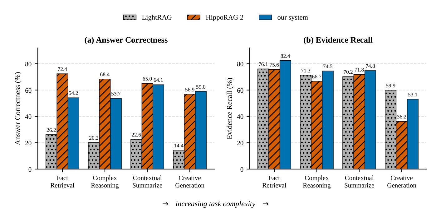
AC across the four difficulty levels on GraphRAG-Bench Medical (all using Meno-Lite-0.1 for graph construction):
| Task | LightRAG | HippoRAG 2 | RAGU |
|---|---|---|---|
| Fact Retrieval | 26.2 | 72.4 | 54.2 |
| Complex Reasoning | 20.2 | 68.4 | 53.7 |
| Contextual Summarize | 22.6 | 65.0 | 64.1 |
| Creative Generation | 14.4 | 56.9 | 59.0 |
The paper says the gap converges monotonically from −18.2 to +2.1, evidence of “stronger as tasks get harder.” But look at RAGU’s own column: 54.2 → 53.7 → 64.1 → 59.0, essentially flat.
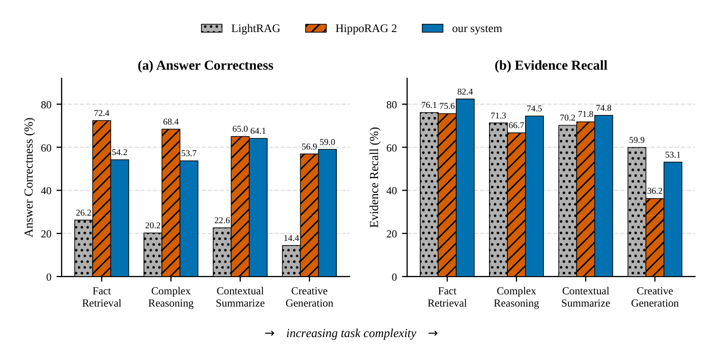
The so-called cross-over is mainly not RAGU getting stronger, but HippoRAG 2 falling from 72.4 to 56.9 — a drop of 15.5 pp. The accurate description would be: RAGU’s performance is insensitive to task difficulty and HippoRAG 2’s is sensitive, so it gets overtaken in the hardest cell. “Stronger on hard tasks” and “degrades less on hard tasks” are two different things, and the paper’s narrative states the latter as the former. Besides, the win in that final cell is 59.0 against 56.9 — 2.1 pp, within the noise range of an LLM judge.
8 Idea three: good retrieval metrics do not mean good answers
One set of numbers here is real. Coverage on Creative Generation: LightRAG 3.9, HippoRAG 2 34.7, RAGU 57.4. RAGU’s Evidence Recall across the four levels is 82.4 / 74.5 / 74.8 / 53.1, higher than both LightRAG and HippoRAG 2 in all four cells. (The absolute values declining with difficulty is the task getting harder, and does not affect who leads.) A 22.7 pp Coverage gap is not noise and is not caused by format; it genuinely supports the paper’s mechanistic hypothesis that consolidation makes the graph more complete and more connected, so more relevant material can be retrieved.
But this raises the tension most worth thinking through in the whole paper: if RAGU retrieves more complete evidence, why is its final answer accuracy worse?
The key is that Evidence Recall only measures “did we retrieve what we should have,” and never measures “did we also retrieve what we shouldn’t have.”
Recall    = relevant material retrieved / all relevant material   ← ER measures this
Precision = relevant material retrieved / all material retrieved  ← nobody measures this
Both can happen at once:
HippoRAG 2's context:  [rel][rel][rel]
   → ER = 3/4 = 0.75    precision = 3/3 = 1.00

RAGU's context:        [rel][rel][rel][rel][noise][noise][noise][noise]
   → ER = 4/4 = 1.00    precision = 4/8 = 0.50
What RAGU retrieves is not “more correct information,” it is “more complete but lower-concentration information.” And this is not an accident, it is a design consequence: consolidation merges all mentions of an entity together, and LocalSearch then expands from entities to relations and on to chunks, so the whole route is biased toward retrieving more. Leading Coverage by 22.7 pp is, read the other way, evidence that it swept a lot of things in.
There are three mechanisms by which retrieving more actually hurts the answer. First, distractors: a factoid question has only one correct answer, and stuffing several more semantically related passages with different answers into the context raises the odds the LLM picks wrong. Second, lost in the middle: in a long context the model is sensitive to the beginning and end and easily overlooks the middle, so “the answer is in the context” and “the model uses it” are two different things — ER measures the former, AC the latter. (How to decide how much to retrieve is exactly the trade-off Adaptive-k tackles.) Third, task nature determines who pays:
| Fact Retrieval | Creative Generation | |
|---|---|---|
| Needs | One precise fact | Broad relevant material |
| Extra material is | A distraction | An asset |
| Favours | High precision | High recall |
This is the real mechanism behind the cross-over. RAGU does not get smarter on hard tasks; it uses one strategy throughout (retrieve more), and that strategy is a burden on easy tasks and only becomes an advantage on synthesis-type tasks.
The paper covers this in a single sentence: HippoRAG 2 still wins factoid AC despite lower Evidence Recall, reflecting the precision of its chain traversal on single-fact queries. The direction is right, but there is no data behind it. And the most critical gap is here — the paper’s list of metrics used includes Context Relevancy, exactly the number needed to answer this question, yet it appears nowhere in any table or figure, with not a single value anywhere in the paper, and no explanation is given.
This idea holds beyond this paper: optimizing recall and optimizing final correctness pull against each other on factoid tasks. Watching only recall-type metrics (retrieval rate, hit rate) systematically pushes a system toward “retrieve more,” while final answer quality may stay flat or even drop. At minimum, watch context precision alongside it; better still, look directly at end-to-end answer metrics.
9 Meno-Lite-0.1: an awkward result
Measured on information extraction alone, the 7B Meno-Lite-0.1 does beat 32B:
| Model | Size | NER | Def | RE | RDef | HM |
|---|---|---|---|---|---|---|
| Meno-Lite-0.1 | 7B | 0.504 | 0.527 | 0.347 | 0.558 | 0.468 |
| Qwen2.5-32B | 32B | 0.536 | 0.528 | 0.239 | 0.599 | 0.416 |
| Qwen2.5-14B | 14B | 0.510 | 0.518 | 0.222 | 0.583 | 0.396 |
| Qwen2.5-7B | 7B | 0.477 | 0.479 | 0.192 | 0.541 | 0.356 |
The columns mean: NER is entity recognition (F1), RE is relation extraction (F1), Def and RDef are description-generation quality for entities and relations respectively (chrF++), and HM is the harmonic mean of all four. The overall HM is 12.5% higher in relative terms, driven mainly by the relation-extraction column (0.347 vs. 0.239).
The problem is that this advantage vanishes end-to-end. The paper writes it itself: Meno-Lite-0.1’s large standalone extraction advantage compresses to within 1 pp on GraphRAG-Bench’s end-to-end QA. The configuration table in the appendix is even more direct — swapping extraction models from 3B to 14B changes final AC by less than 1.5 pp.
The same body of evidence proves both “small models are enough” and “it barely matters which extraction model you use,” which incidentally thins out Meno-Lite-0.1’s own reason to exist. The paper reframes this as robustness of the pipeline.
There is one more caveat the paper concedes in its Limitations: Meno-Lite-0.1’s fine-tuning used NEREL’s train/validation split, while the IE benchmark uses a held-out test split. The paper says the overlap is limited to the annotation schema and text domain, but a residual advantage cannot be fully ruled out.
10 Engineering: the most solid part of the paper
The engineering comparison between RAGU and HippoRAG 2 in the appendix is the part of the paper I admire most. It pins a specific commit and attaches a filename and line number to every accusation (eval() appears at openie_openai.py:36,88; assert False used as control flow at HippoRAG.py:216). That kind of checkability is rare in a paper.
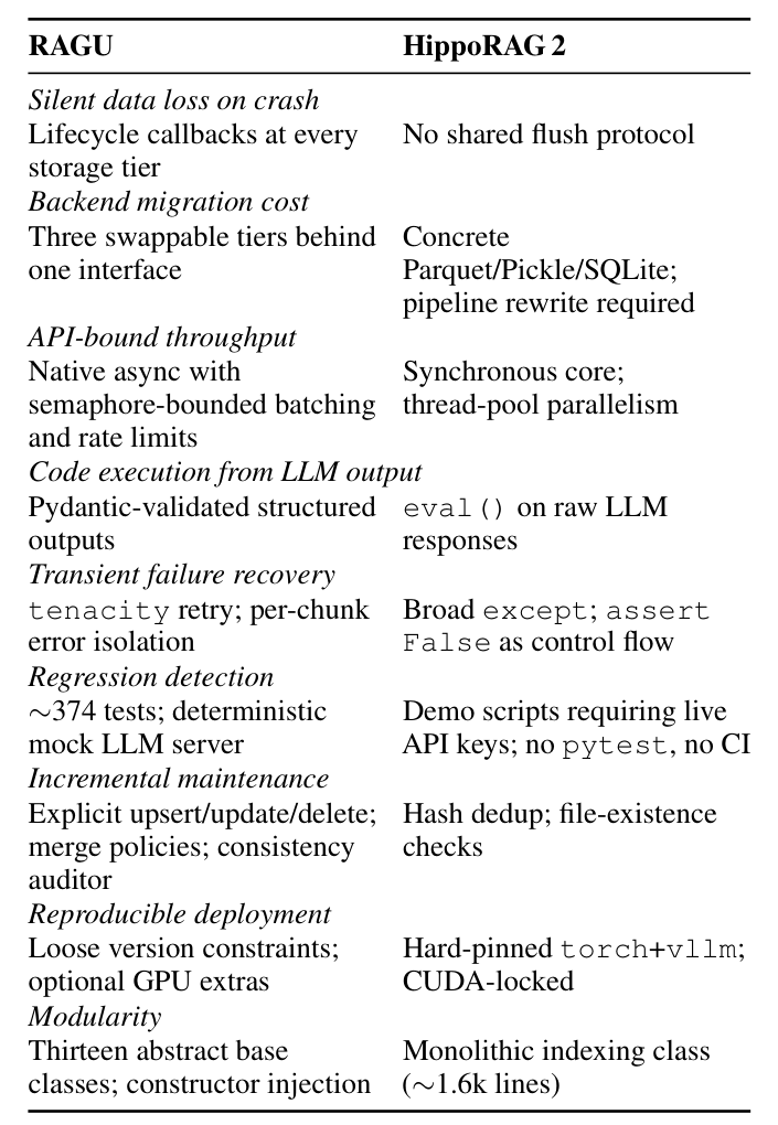
The substance on RAGU’s side:
- Three swappable storage tiers (NetworkX → Neo4j, NanoVDB → Qdrant, changing only two constructor arguments)
- Async-first API with bounded concurrency control
- Pydantic v2 validation for all structured LLM output, replacing
eval()and eliminating code injection - Incremental upsert / update / delete, deterministic hash IDs, consistency auditing
- Around 374 tests with a deterministic mock LLM server, so CI needs no API key
Frankly, the value of this section is reference-manual grade: if you ever actually need to build GraphRAG, this is an implementation you can install and whose backends you can swap, which beats writing it from scratch. But it is not knowledge you need to hold in your head.
The paper’s self-declared limitations are honest too: the default NetworkX backend will not hold up on million-node corpora; the NEREL schema was designed for Russian news and needs redesigning for a new domain; and structural noise introduced by a weak extraction model cannot be rescued by consolidation.
11 Five things worth taking away
The paper’s own research contribution is close to zero, but the following points are durable, ordered by value.
1. Good retrieval metrics do not mean good answers. ER measures recall only, not precision. Watching hit rate alone systematically pushes a system toward “retrieve more,” while final answer quality may stay flat or even drop. This one changes which dashboard you watch when tuning a system, and it has nothing to do with GraphRAG.
2. A sense of scale for confounders. Changing the generation prompt is worth +16.9 pp AC, more than all of this paper’s methodological contributions combined. Before evaluating any retrieval change, ask: is there a more boring variable (prompt, answer format, chunk size, baseline configuration) explaining this difference?
3. A useful negative result. RAGU against NaiveRAG — same code, same prompt, the only difference being whether a graph is used — comes out at +1.2 to +4.3 pp. That is what the entire GraphRAG stack is worth. Knowing what not to do is as valuable as knowing what to do, and numbers like this are rarely published.
4. Two conceptual tools. Entity resolution is not clustering — judging identity vs. discovering structure, k≈n vs. k«n, bad merges being irreversible — and that decides whether you pick union-find or DBSCAN. And graph clustering and vector clustering are two kinds of “similar” — structural relatedness vs. semantic similarity — both of which get used in the same pipeline.
5. A set of checks for reading papers. This paper trips all three, which is the fastest way to judge its quality: find the “clean comparison” (which two things differ by exactly one variable), which here is NaiveRAG; look for “metrics declared but never reported,” which here is the missing Context Relevancy; and check whether the core selling point has an ablation, which here consolidation does not.
12 Conclusion
RAGU is a system paper with high engineering value and low research value. Its two-stage typed extraction is a good pattern you can take away on its own, and its engineering quality is unusually solid among comparable open-source projects. But its core selling point, consolidation, never gets an ablation; the “7B is enough” hypothesis is a post-hoc justification for a decision already made; and the prettiest narrative, the cross-over, on inspection is mainly the competitor falling rather than RAGU climbing.
What is genuinely worth remembering is that it inadvertently quantified GraphRAG’s ceiling — using its own code and its own prompt as the control, the entire graph’s net contribution is only 1.2 to 4.3 pp, and that ceiling is a lot lower than advertised. For anyone currently evaluating whether to adopt GraphRAG, that is far more useful than what the paper set out to prove.