Do Self-Improving Agents Just Memorize the Test? Inside Google's RRSI

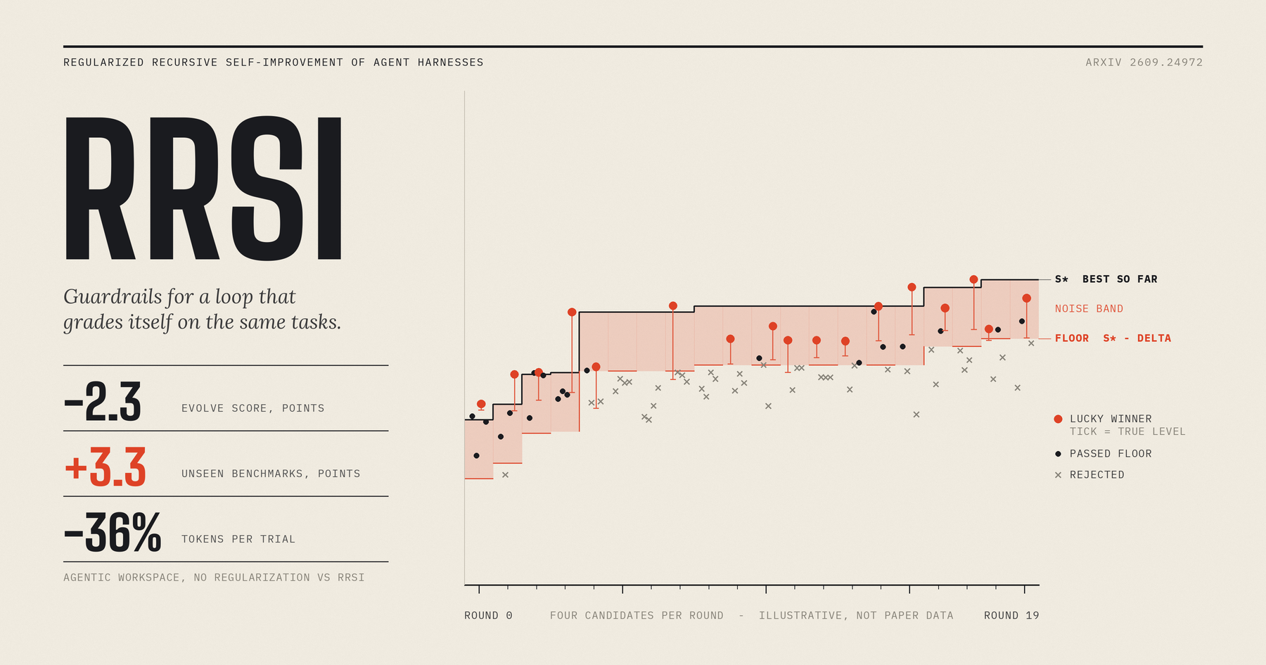
1 Introduction
Letting an LLM automatically rewrite an agent’s harness (everything outside the model: prompts, control flow, tool interfaces, memory and context management), then using task scores as feedback to iterate, has become a popular recipe over the past year or two. The catch is that every round is scored on the same limited set of tasks. The score on the evolution tasks climbs steadily, but on benchmarks the system has never seen, the gain shrinks or vanishes.
RRSI (Regularized Recursive Self-Improvement of Agent Harnesses, arXiv 2609.24972v2) from Google Cloud AI Research tries to rein this in. It does not restrict what a harness may change. It governs how modifications are proposed and which ones are allowed to stay, using a bundle of rules to reduce overfitting.
This article has two halves. The first follows the paper’s order: the problem, the method, the experiments and an evaluation. My verdict is low research value and medium-to-high engineering reference value. The second half is nine extension concepts. Adaptive data reuse, the winner’s curse, L0 / L1 / L2 regularization and the noise band hold up independently of this paper, and I think they are the part most worth keeping. The rest are open questions the paper leaves behind.
If you only have five minutes, read “Overall Assessment” and “Conclusion”. To understand the method, read through the selection side. To judge whether the paper is trustworthy, read “Experiments and Results” and “Overall Assessment”.
Reading markers: “made-up example” means numbers or scenarios the paper does not contain, which I invented to explain a mechanism. “Inference” means my own judgement, which the paper does not state. “Not stated in the paper” means a detail the paper leaves out, and I do not fill it in here.
2 The Problem: Why Automatic Harness Evolution Overfits
Having an LLM improve a harness automatically looks like a loop that steadily gets better, but it has a structural flaw: every round’s decisions reuse the same limited set of tasks, so the “progress” may just be memorizing those tasks.
2.1 Agent, Harness and “Evolution”
The paper splits an agent into two parts: a backbone model whose weights never change, and a harness wrapped around it. The harness is everything outside the model:
- the system prompt and task prompts
- control flow: when to plan, act, reflect or stop
- tool interfaces and tool descriptions
- memory and skill files
- context management: what the model gets to see at each step
For the same model, how well the harness is designed decides whether it reads a file before editing it, whether it can recover after a failed command, whether its context overflows, and whether it finally writes the result into the deliverable. In the past all of this was adjusted by hand after an engineer read the failure logs, so progress was capped by how many logs an engineer could read in a day.
Harness evolution automates that manual loop: another LLM (called the proposer) reads failure logs and proposes modifications, and task scores are used to select among them. Because every round uses feedback produced by the “current system” to improve the “next system”, the paper calls it RSI (recursive self-improvement) at the level of the agent system, except that what changes is the harness, not the model weights.
One round of evolution goes as follows:
- The current harness runs on the evolve set (the tasks used for evolution).
- This produces trajectories (one complete execution record per task), which are organized into failure feedback (written up by a separate analyst LLM).
- The proposer generates a few candidate harnesses from .
- The candidates are re-scored on the same evolve set.
- Among the candidates plus the original , the highest scorer becomes the next round’s , and the loop returns to step 1.
As a formula (paper Eq. 2):
- : the incumbent harness in round .
- (calligraphic H): the set of candidates the proposer generates this round.
- : the unconstrained proposal distribution, meaning the proposer may change whatever it likes.
- : this round’s failure feedback (Concept 5 in the extensions explains what it is).
- : the measured score. The hat means it was run only a finite number of times and carries random noise.
- : finds the candidate that maximizes the quantity after it, and returns the candidate itself, not the score.
Note that the range of includes itself: if no candidate beats the current one, stays in place and nothing changes this round.
2.2 The Core Problem: Adaptive Overfitting
Steps 1 to 4 above keep reusing the same evolve set, and what to change next depends on results measured on that same set in earlier rounds. Statistically this is called adaptive data reuse: the set is no longer independent test data but data the search process has “seen” step by step. The result is that the evolve-set score keeps rising, while on tasks it has not seen the gain shrinks sharply, and can even end up worse than the original harness with no changes (written ). In short, each round’s decision rests on results from this set, so the score on this set is no longer trustworthy. The principle is covered in Concept 1 at the end.
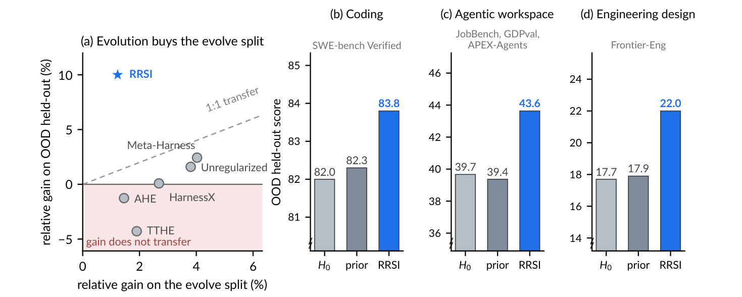
Figure 1 has several subplots. We look at (a), the results on agentic workspace tasks. The “average of the four opponents” for coding and engineering appears in (b) and (d). The x-axis is the relative gain on the evolve tasks and the y-axis is the relative gain on an unseen benchmark (OOD). A “1:1 transfer” diagonal marks gains that carry over completely. The four existing methods (Meta-Harness, AHE, TTHE, HarnessX) all fall below the line, and some even have a negative y value (the plot labels this “gain does not transfer”). Only RRSI lands above it.
2.3 Three Behaviors That Cause Overfitting
The paper identifies three coupled behaviors that together widen the gap between the “evolve score” and the “score after switching tasks”. The three line up with the guardrails described later:
| Behavior | In plain words | Made-up example | Matching guardrail |
|---|---|---|---|
| benchmark-specific fitting | The modification directly memorizes features of these tasks | A task fails because a company name has the wrong format, so the proposer adds “for Acme’s reports, use format YY” to the prompt. The evolve score rises; on a different batch of tasks it is useless | D (leakage screening) |
| noise chasing | The selected candidate simply got lucky in this scoring | Four candidates all truly score 90.0, and are measured at 89.7, 90.4, 89.9 and 90.1. Picking the highest, 90.4, looks like a 0.4 gain when there is no gain at all | E (score floor), noise band |
| complexity accumulation | Each change adds bulk, and the score comes from spending more compute, not from a better mechanism | In Table 2, evolution with no regularization has the highest evolve score, but uses 2.4 times the tokens of the original harness | F (cost rule), G (structural pruning) |
Two reminders. First, the three behaviors are clearly distinct conceptually, but in practice they probably occur together in the same modification (inference: a modification that hard-codes task features may also make the prompt longer). Second, the paper introduces the three behaviors in a short passage and does not run separate experiments to measure how much each contributes. The later ablation removes the whole set of regularizers at once.
2.4 Terms Used Later
- evolve set: the tasks repeatedly used for scoring during evolution.
- ID held-out (in-distribution held-out): tasks in the same benchmark that were not used during evolution.
- OOD (out-of-distribution): a benchmark never seen during evolution.
- policy: the model that actually executes the tasks. In the paper’s main experiments the policy is fixed to Claude Opus 4.8.
- trajectory: the complete record of one agent run on one task, including each step’s reasoning, tool calls and results.
3 RRSI Method Overview
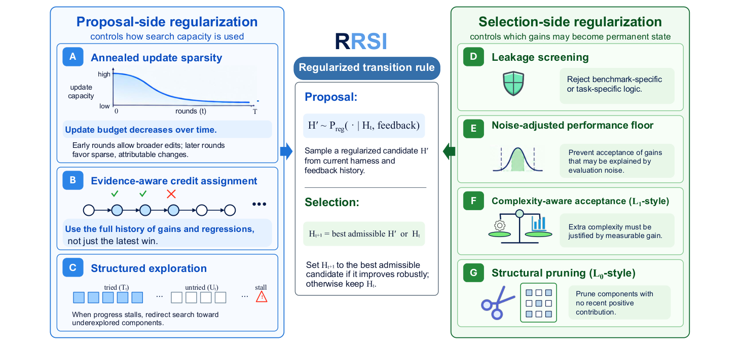
RRSI does not shrink the range of what a harness can change at all. It governs just two things: how the proposer produces modifications (the proposal side), and which measured improvements are allowed to become permanent state (the selection side).
3.1 Understanding It as a Code Review Process
Think of the harness as a repo and each round of evolution as one pull-request process:
- No restriction on what can change: any file in the repo may be touched. Prompts, tools, memory, control flow and subagents can all be changed. The paper uses for “every harness reachable from by editing arbitrary source code”, and deliberately keeps it open.
- The proposal side is the rules for “how to submit a PR”: a PR changes at most a few things (A), you review past rejected PRs before submitting (B), and when there has been no progress for a long time you must touch modules nobody has touched (C).
- The selection side is the merge gate: a higher CI score is not enough. The change must not hard-code test answers (D), must not be a flaky test getting lucky (E), and must not blow up build time without a matching benefit (F).
- Permanent state is merging into main: the selected becomes the starting point for every later proposal, so a wrong pick compounds through every following round.
The analogy breaks down in one place. A real code review has independent people and independent tests, while RRSI’s “CI” is just the score on the same evolve set, which is itself noisy and gets reused again and again. So D, E and F patch holes, but cannot replace independent validation (inference).
3.2 The Seven Components
| Code | Name | What it does | Problem it targets |
|---|---|---|---|
| A | annealed update sparsity | Limits how many modifications one candidate may bundle, decreasing with the round number | Bundling too many modifications means high capacity and hard attribution |
| B | evidence-aware credit assignment | Records the outcome of every modification for later proposals to consult | Avoid retrying ideas already rejected |
| C | structured exploration | When progress stalls, reserves slots for component categories not yet tried | Proposals concentrating on one kind of change (for example always editing the prompt) |
| D | leakage screening | Before scoring, a critic (an LLM in charge of review) reads the modification and blocks ones that hard-code task information | benchmark-specific fitting |
| E | noise-adjusted performance floor | A candidate’s score must be the historical best | noise chasing (what it actually blocks is consecutive small regressions, see Concept 4) |
| F | complexity-aware acceptance | Extra tokens must be paid for with score gains | complexity accumulation |
| G | structural pruning | Components with no positive contribution for a while are listed as deletion targets | complexity accumulation |
The mapping of D through G to the three behaviors is stated by the paper itself at the start of Section 3.3. For A through C the paper gives reasons but no item-by-item mapping. My inference: A through C reduce overfitting-prone proposals at the “source”, and D through G check them at the “exit”.
The two-sided split is only a conceptual classification, not a division of code. Algorithm 1 (the proposal side) already contains D’s pre-scoring screening and G’s pruning-target computation.
3.3 The Transition Rule: Only Two Changes From the Old Rule
The old rule (Eq. 2) selects among “all candidates plus ”. RRSI’s version (paper Eq. 8):
If no candidate passes (the intersection is empty), then .
- : the constrained proposal distribution. It is really just the proposer LLM, with extra inputs listed below.
- : the history of all past modifications (component B).
- : the maximum number of modifications each candidate may bundle this round (component A).
- : the exploration instruction, which says to try untried components when stalled (component C).
- : the deletion targets from structural pruning (component G).
- : the admissible set, meaning the candidates that pass every gate, with D, E, F and the domain guard deciding who gets in.
- : intersection. Only candidates that are both “a candidate” and “admissible” may compete.
So only two things changed: the proposal distribution goes from the unrestricted to the restricted , and the pool for picking the highest score shrinks from all candidates to those that passed the gates, with the incumbent kept if none survive.
Made-up example: scores 90.0 and there are three candidates this round. X scores 91.0 and is blocked by D (hard-coded task information). Y scores 90.8 and is blocked by F (cost rose too much). Z scores 90.5 and passes everything. The old rule picks X, and RRSI picks Z. If Z had not passed either, and nothing would change this round.
3.4 Why It Is Called “Regularization”, and Why It Is Not Traditional Regularization
Traditional regularization adds a penalty term to the optimization objective, limiting what shape the model can take. RRSI cannot do that: the candidate space of harnesses is heterogeneous. One candidate edits a prompt, another adds a subagent, a third changes control flow, and none of these fit into one parameter vector, so there is no way to define “how large the parameters are”. The paper says plainly in Appendix C that it does not optimize any norm-penalized objective.
So RRSI instead restricts how the search proceeds step by step: it leaves the hypothesis space alone and governs only the proposal rule and the acceptance rule. The paper calls A L0-style, G L1-style and F L2-style. This is just a metaphor, and the names do not bring sparsity or shrinkage properties. See Concept 3.
4 The Proposal Side: A, B, C
The ablation in Table 2 only removes the whole group; no component is validated individually, and the sections below do not repeat this. All three proposal-side components are inputs handed to the proposer. Only A has a concrete number. B and C are information fed to an LLM, and the paper does not describe how it makes sure the proposer follows them.
4.1 A: Annealed Edit Budget
The proposer can bundle many unrelated modifications into one candidate. The more it bundles, the easier it is to fit the quirks of the current batch of feedback (high capacity), and when the score changes you cannot tell which modification caused it (hard attribution).
RRSI’s approach is to cap each candidate each round at “independently attributable modifications”, with decreasing over the rounds. Early on, bundling several modifications is allowed so the search can explore new mechanisms, and later the cap tightens step by step. This is a learning-rate-scheduler-style schedule, except that what is scheduled is “how many things can be changed at once”. Paper Eq. 4:
is the round number (starting from 0), is the total number of rounds, is the starting budget, is the ending budget, and rounds up. The coefficient in the middle falls smoothly from 1 to 0, so falls from to (derivation in Concept 6).
Using Table 5’s coding setting (, , ) and computing all 20 rounds (calculated from the formula, not listed in the paper):
| Round | Budget | How many rounds |
|---|---|---|
| 0 to 7 | 4 | 8 rounds |
| 8 to 12 | 3 | 5 rounds |
| 13 to 19 | 2 | 7 rounds |
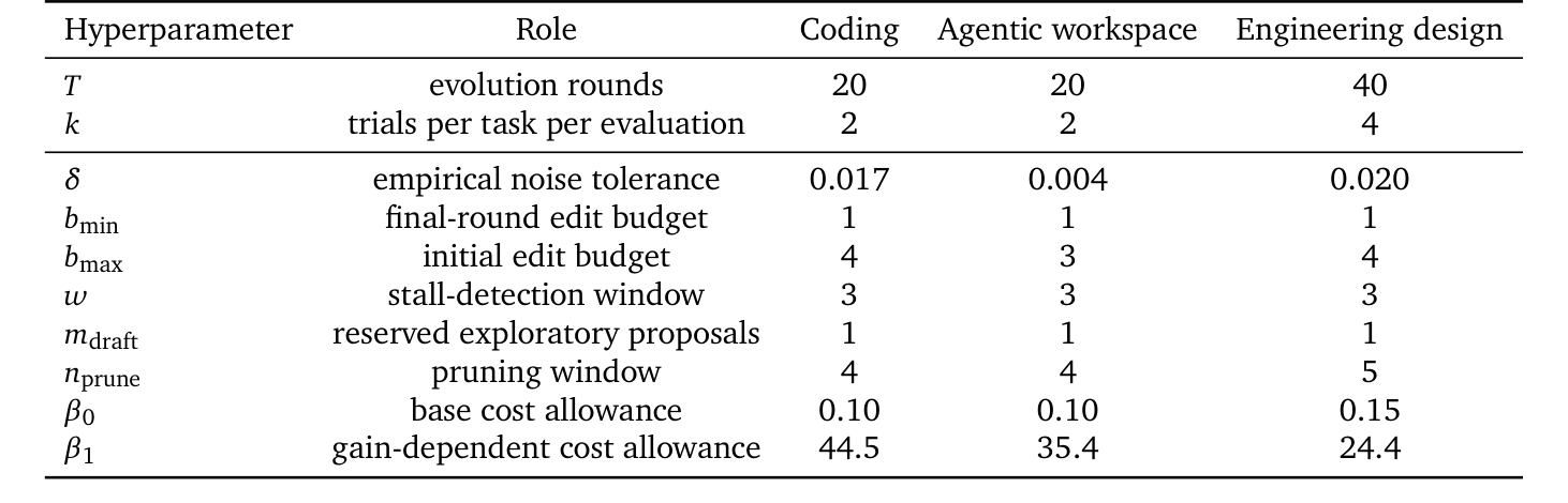
A real example in the paper is in Table 6 (Coding R0-A): in round 0 the candidate added both a “verification check before completion” and “non-blocking polling guidance for long-running tasks”, the evolve set gained 3.93 points, and it was accepted. The round-0 budget is 4, so bundling like this is allowed.
The formula and the paper’s hyperparameters yield two findings:
- The budget never reaches . When the coefficient is always greater than 0, so the value before rounding up is always greater than 1, and the minimum is 2. would only occur at , but Appendix C.1 says one evolution runs only to . The final rounds for agentic and engineering are also 2. Yet Table 5 labels as “final-round edit budget” with the value 1. There are two readings: taken literally, the formula still lets the last few rounds bundle two modifications, so attribution is not as clean as the paper claims. Or the implementation rounds or numbers rounds differently and the last round really is 1. The paper’s text cannot settle which.
- The cosine shape is almost packaging. After rounding, the whole schedule has only three steps, 4, 3 and 2, which is substantively no different from a step function of “4 for the first 8 rounds, 3 for the middle 5, 2 for the last 7”. The cosine only decides in which round the steps switch, and a linear decrease would give nearly the same result (inference). The paper also does not ablate the schedule shape or the “annealing” separately.
4.2 B: Evidence-Aware Credit Assignment (History)
B writes an “experiment record” for every evaluated candidate, and every later round lets the proposer read it, so it avoids retrying failed ideas and remembers ideas that worked. The record format (paper Eq. 10):
Each record is a 7-tuple:
- : the round in which this modification was proposed.
- : the component category of the modification, for example prompt, control_flow, memory, subagent.
- : the hypothesis this modification tries to test.
- : the actual code difference (source diff).
- : the score change, the candidate’s score gain relative to the incumbent harness.
- : the cost change, the proportional increase in token cost.
- : whether it was adopted. means the candidate this modification belongs to won that round. covers every other case, including candidates blocked by the rules and candidates that passed the rules but lost to a higher-scoring candidate (stated explicitly in Appendix C.2).
- : the total number of records accumulated before round .
If a candidate bundles several modifications, each modification gets its own record, but they share the same , and outcome.
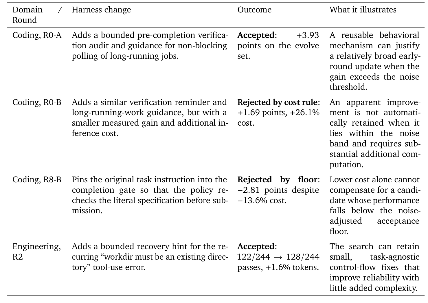
Here are three entries from Table 6 rewritten as records:
| Case | Modification | |||
|---|---|---|---|---|
| Coding R0-A | A pre-completion verification check, plus non-blocking polling guidance for long tasks | +3.93 points | Not listed in the paper | 1 |
| Coding R0-B | A similar verification reminder, plus long-task guidance | +1.69 points | +26.1% | 0 (rejected by the cost rule) |
| Engineering R2 | A recovery hint for the “workdir must be an existing directory” error | 122/244 to 128/244 passes | +1.6% | 1 |
Credit assignment comes from reinforcement learning. The question is “when a reward arrives only after a sequence of actions, how should credit be split among the actions”, and it is often traced back to Minsky 1961 (general knowledge, not from the paper). The paper stretches the term a little: what is actually done is just “keep an experiment log for the proposer to read”, with no computation of each modification’s individual contribution.
A few doubts and limitations:
- Bundled modifications do not get their credit truly separated. R0-A’s two modifications (reading it as two modifications is my interpretation) each get a record with +3.93, which looks like each improved by 3.93 when really they only improved by 3.93 together. This ties B’s quality to A.
- mixes two meanings: “blocked by a rule” and “lost to a better candidate in the same round”. The latter does not mean the idea failed. R0-B is an example: its hypothesis direction is the same as R0-A’s, and it was rejected because it gained only +1.69 while costing 26.1% more, which means “this version is not worth it”, not “the verification reminder is useless”. The paper does not say how the proposer tells the two apart.
- The paper does not say how the proposer “conditions on this history” (is the whole log put in the prompt, or summarized first), nor who assigns the labels and .
- Candidates blocked by the critic before scoring have no measurement and may not be in the log (Concept 8).
- “Showing the history to the proposer” is not new. The baselines Meta-Harness and AHE described in Appendix B already do something similar, so B’s only difference is a more structured format, which the paper does not measure separately, and Table 2 does not remove B on its own either.
4.3 C: Structured Exploration
C is an anti-fixation rule: when the search makes no progress for several consecutive rounds, the stall signal and a list of “component categories not yet touched in this evolution” are handed to the proposer, and one candidate slot is reserved for exploration. The paper’s example is a proposer that keeps rewriting the prompt while the agent’s structural mechanisms (tools, memory, subagents) are never touched. B lets the proposer see the history, but the history alone does not guarantee that it will try new directions.
The mechanism is in paper Eq. 13 and Appendix C.2:
- : the score of the incumbent harness in round . : the window size for stall detection, looking at the most recent rounds.
- : the noise band (Concept 4). A gain that does not exceed it is treated as indistinguishable from noise.
- : equals 1 if the condition inside holds, otherwise 0. means “stalled”.
- : the full set of component categories, 9 in total: prompt, control_flow, config, output_plumbing, context_mgmt, client_tool, skill, memory, subagent.
- : the categories that so far have at least one measured modification. is minus , that is, the categories not yet touched.
- : the number of candidate slots reserved for exploration when stalled.
Walking through it once with Table 5’s coding setting (, , ) and made-up scores: and , a difference of 0.012, which does not exceed 0.017, so and the search is judged stalled. If , the difference is 0.025, greater than 0.017, so and nothing triggers. Suppose the first 8 rounds touched prompt, control_flow and context_mgmt. Then is the other 6 categories, and the proposer receives this list and is asked to reserve 1 candidate slot for them.
Doubts and limitations:
- The paper does not describe how it ensures the proposer complies. The wording is only reserved and redirect, with no enforcement mechanism (Concept 7).
- The “not yet touched” test is crude: touching prompt once counts as tried regardless of which part was edited, and rejected modifications count too.
- Inference: has only 9 categories and each round has several candidates, so may empty quickly, and the paper does not say what happens then.
- Who labels the component categories (the proposer, code, or another analysis LLM) is not stated in the paper, and C’s decision depends entirely on those labels.
- Table 6 has no example of a stall trigger either, so there is no evidence it has any effect.
4.4 Overall Judgement on the Proposal Side
A, B and C are three soft instructions to an LLM, and only is an explicit number. The directions are all reasonable and easy to implement, but the paper does not prove that each one works on its own. The only evidence for the whole proposal side is one row of Table 2, “w/o proposal regularizers”. My inference is that B is most likely to help, because showing past results to the proposer is what every baseline already does, while the effects of A and C are the least certain.
5 The Selection Side: D, E, F, G and the Final Choice
The selection side is a series of gates, each blocking a different thing. A candidate must pass all of them in order, and the highest scorer among the survivors is chosen. Each gate is sensibly designed, but none has been validated on its own.
5.1 D: Leakage Screening
Before a candidate is scored, a critic (an LLM dedicated to review) reads its code difference (diff) and keeps out modifications that “hard-code task information”. What the paper states explicitly (Section 3.3, 4.1, Appendix C.3):
- What it blocks: explicitly written task names, entity names, task-specific values, answers, or other logic that holds only for the evolve benchmark. It also blocks “inert machinery” (code that was added but does nothing).
- It governs content, not component category: general improvements to prompts or tool descriptions can still pass.
- The timing is before scoring. The reason is that a blocked candidate never gets the high evolve-set score that would make it look attractive.
- The executor is Claude Opus 4.8, the same model as the proposer and the analyst.
Leakage comes from data leakage in machine learning, where information from the test data seeps into training and distorts evaluation. The term fits well here and is not just packaging: if a candidate writes the evolve tasks’ answers into the harness, the grading criteria have leaked into the thing being graded, and the evolve score is inflated.
Made-up example: candidate P adds to the prompt “for Acme’s merger contracts, always write the penalty clause as 15%”, and is blocked (hard-coded entity name and value). Candidate R adds a helper function that is never called, and is blocked (inert machinery). A real example that passes is Engineering R2 in Table 6: for the repeatedly occurring tool error “workdir must be an existing directory”, it adds a bounded recovery hint. It contains no task information and was accepted (122/244 to 128/244 passes, only 1.6% more tokens), and the paper uses it as its representative task-agnostic fix.
Doubts and limitations:
- The critic’s criteria and prompt are not published, and there is no adjustable threshold, so the line between “general” and “specific to this benchmark” is entirely the LLM’s judgement.
- It only blocks explicitly hard-coded content. A modification that hard-codes no names but happens to fit the evolve tasks’ distribution (for example assuming every task needs a summary table) is unlikely to be caught by the critic (inference).
- The critic and the proposer are the same model, so their blind spots may overlap heavily (inference).
- None of the cases in Table 6 was blocked by the critic, and the paper does not report the fraction it blocks.
5.2 E: The Noise Band δ and the Score Floor
Before evolution starts, the unmodified is scored repeatedly to see how much its score naturally wobbles, and that size is . After that, no candidate’s score may fall below “the historical best minus ”.
The paper gives only one sentence about the method (evaluate the unmodified base harness repeatedly before evolution to estimate an empirical noise band), and stays fixed afterwards. The paper gives results for three domains with the matching actual counts (Table 5, Appendix D.1), and I checked the arithmetic: 3/178 0.0169, 60/14,100 0.0043, 5/244 0.0205, consistent with the table.
| Domain | Corresponding actual count | |
|---|---|---|
| coding | 0.017 (1.7 points) | 3 passes out of 89 tasks × = 178 trials |
| agentic workspace | 0.004 (0.4 points) | 60 grading items out of about 14,100 |
| engineering design | 0.020 (2.0 points) | 5 passes out of 61 tasks × = 244 trials |
In the table, is how many times each task is repeated per evaluation, and a pass is a passing trial. The paper does not say how many times it repeats the evaluation before evolution, or which statistic it uses for (standard deviation, range or some quantile).
The score floor (paper Eq. 5):
is the measured evolve-set score of candidate . is the highest evolve score observed so far over the whole evolution, starting at and updated each round to . It is a necessary condition for accepting a candidate and cannot be offset by other terms (the paper calls it non-compensatory). Coding R8-B in Table 6 is the only instance: pinning the original task instruction into the completion gate gave a score of and a cost of , and since coding’s is 1.7 points, the drop exceeds it and saving cost cannot rescue it.
The floor is tied to the historical best rather than the incumbent harness to stop the search from “walking downhill continuously”: each step’s regression is small enough to pass as noise, but accumulated they add up. A numeric example is in Concept 4.
There is an easily overlooked fact about this gate: what it guards against is not actually “fake progress”. Section 3.3 of the paper describes E using noise chasing, but Eq. 5 sets only a lower bound, and what it blocks is consecutive small regressions. A candidate that merely got 0.3 extra points by luck will not be stopped. To really block lucky fake progress, the statistically more sensible rule is to require , at the price of wrongly rejecting real gains that were unlucky. Concept 4 covers the tradeoff between the two.
Other doubts:
- was measured only once on and then applied to all candidates, and the paper does not validate that assumption. The evolved harness takes more steps (Figure 4(b): 21.2 steps rising to 26.3), so its noise may not match ’s (inference).
- records the measured score of the selected candidate, and the selected one is the highest, so it may be inflated by luck (the winner’s curse: the highest of several noisy scores is usually inflated by luck, see Concept 2).
- Algorithm 2 does not say whether the incumbent harness’s score reuses the measurement from when it was selected or is re-measured every round.
5.3 F: The Cost Rule (Candidates Whose Gain Exceeds δ)
F’s principle: extra tokens must be paid for with score gains, and the more the gain, the more extra cost is allowed. First two quantities are defined (paper Eq. 6), then the rule (Eq. 7):
- : how many more points the candidate scores than the current incumbent, expressed as a fraction (7 more tasks out of 178 = 0.039). Note it is compared with the incumbent harness, not the historical best.
- : the relative change in average policy tokens per trial. 1.0M becoming 1.5M is 0.5, and becoming cheaper gives a negative number.
- : the base allowance, given regardless of gain (0.10 for coding, i.e. 10%).
- : the exchange rate, how much extra cost increase is allowed per unit of gain (44.5 for coding).
In plain words: allowed cost increase = base allowance + exchange rate × score gain. If the actual cost increase does not exceed that allowance the candidate passes, and otherwise it is rejected.
Made-up example with coding’s settings (, ):
| Candidate A | Candidate B | |
|---|---|---|
| Extra tasks passed | 7 | 4 |
| 7/178 = 0.039 | 4/178 = 0.022 | |
| Allowed cost increase | 0.10 + 44.5 × 0.039 = 1.85 (185%) | 0.10 + 44.5 × 0.022 = 1.10 (110%) |
| Actual cost increase | 50% | 150% |
| Result | 50% 185%, passes | 150% 110%, rejected |
Gaining 7 tasks for 50% more cost is worth it. Gaining 4 tasks for 150% more is not.
What actually means (Appendix D.1, I checked the arithmetic): coding’s amounts to allowing 25% more tokens per additional task passed. Agentic’s is 25% more per additional 100 grading items. Engineering’s is 10% more per additional task passed. is 0.10, 0.10 and 0.15 respectively.
Doubts and limitations: the allowance is very generous and is computed relative to the incumbent, with no absolute cap relative to . Accepting three candidates in a row that each cost 30% more compounds to , about 2.2 times (arithmetic). There is no sensitivity analysis for how was chosen.
5.4 Candidates Whose Gain Falls Inside the Noise Band (Eq. 17)
Candidates whose gain does not exceed (including small regressions) skip the cost cap and use an additive formula to decide whether to keep them:
- , : as above. is positive for a gain, and is positive when more expensive and negative when cheaper.
- : among the structural components this candidate touches (the four categories client_tool, skill, memory, subagent), how many have never appeared in an “adopted modification”.
- , , : the weights of the three terms.
In plain words: gains add points, extra cost subtracts, trying a new structure nobody has succeeded with adds, and the candidate passes if the total is greater than 0. Coding sets , so score change counts for nothing in this rule, and the formula reduces to .
Made-up example, three coding candidates, all inside the noise band and all passing the score floor:
| Score | Cost | Touches new structure | Formula | Result | |
|---|---|---|---|---|---|
| P | +3 tasks | +26% | No | Rejected, whatever the weights | |
| Q | Flat | No | Passes (as long as ) | ||
| R | Flat | +5% | First memory addition | Passes only if |
P is Table 6’s Coding R0-B (+1.69 points, +26.1% cost, rejected). R0-B gained 3 tasks, and coding’s is about 3 tasks (1.7 points), which does not count as “exceeding”, so it takes this rule. This is what I got by matching numbers, and the paper does not state it.
Doubts and limitations:
- The paper says , and are listed in Table 5, but the actual Table 5 does not have them, so how strong the novelty bonus is cannot be known.
- The branch boundary is a cliff. In coding, passing 3 more tasks while costing 26% more is rejected. Passing 4 more ( exceeds , switching to Eq. 7) allows about 110% more cost, and even an 80% increase passes. The difference between 3 and 4 tasks is 0.56 points, far smaller than the noise band itself.
- This rule is a harder push toward exploration than C, because it directly changes who gets accepted. But it only governs candidates inside the noise band, and only works for the four structural component categories.
- Why coding sets , and whether it was done to let small gains through, is discussed in Concept 9.
5.5 G: Structural Pruning
If a component category has produced no gain in its recent modifications, it is listed as a deletion target and handed to the proposer, asking it to propose “remove this kind of thing”.
- : the component category, 9 in total. : the score change of the -th record (record format in B).
- : look only at records from the last rounds (4 for coding, 5 for engineering).
- : the best score change this category had in recent rounds.
- : the categories modified at least once so far. is those categories with , i.e. the pruning targets.
In plain words: if in the last 4 rounds even this category’s best attempt produced no gain (less than or equal to 0), it goes on the deletion list. Made-up example, round 8, , looking only at records from round 4 on:
| Component category | Records (round: score change) | Best in window | Result |
|---|---|---|---|
| memory | Round 3 +0.02, round 5 , round 6 0.00 | 0.00 (round 3 is outside the window) | Listed as a deletion target |
| skill | Round 6 +0.01 | +0.01 | Kept |
It is only a suggestion, not a forced deletion. At the start of each round, code computes from the history and puts it into the proposer’s input, and Appendix C.2 says the proposer is instructed to remove mechanisms that produce nothing. The code never deletes anything directly. After the proposer proposes a deletion candidate, it still has to pass every gate. So the cost of a mistaken listing is only that the proposer wastes a proposal slot: if the component was actually useful, the score drops after deletion and E blocks it. If deleting has no effect and saves cost, the candidate even earns extra credit in the cost rule.
Doubts and limitations:
- The formula defines the maximum of an empty set as negative infinity, so a category that “was tried before but has no records at all in the window” would, read literally, also be listed. Appendix C.2’s text, however, says “recently touched but without gain”, and the paper does not decide which it is.
- “Component” here is 9 broad categories, and the paper does not say whether what actually gets deleted is a whole category or some portion within it.
- G is placed on the selection side in Figure 2 and Section 3.3, but in Algorithm 1 the pruning targets are computed on the proposal side and carried out by the proposer.
5.6 Domain-Specific Guard and the Final Selection Rule
Coding and agentic have no guard, so this gate simply lets everything through. Engineering rejects a candidate that meets either condition below, and the rejection cannot be offset by score (Appendix C.3):
- The valid-output rate falls by more than 0.03 relative to the incumbent.
- The no-submission rate rises by more than 0.02 relative to the incumbent.
The intent is to avoid accepting candidates whose “pass rate rises but basic execution validity gets much worse”. Made-up example: the incumbent has a valid-output rate of 0.95, and the candidate’s pass rate improved but its valid-output rate fell to 0.90, a drop of 0.05, over 0.03, so it is rejected. The two thresholds (0.03, 0.02) are not in Table 5, the paper does not say how they were chosen, and the two rates are given only names, without definitions.
For a candidate to be accepted it must pass these gates in order (Algorithm 2):
- D: the critic check (before scoring).
- Score on the evolve set to get and .
- E: the score must not be lower than the historical best by more than .
- If , go through F (Eq. 7), otherwise the in-noise-band rule (Eq. 17).
- The domain guard (engineering only).
- Among all candidates that pass, pick the highest score as and update . If no candidate passes, .
The last step is still “pick the highest score”, so the winner’s curse (Concept 2) is not fully eliminated; the earlier gates just filter out the clearly problematic candidates first.
5.7 Summary Table
| Code | Component | When it checks | What it checks | Problem it targets |
|---|---|---|---|---|
| D | leakage screening | Before scoring | The critic reads the diff, blocking hard-coded task information and code that does nothing | benchmark-specific fitting |
| E | score floor | After scoring | Score historical best | The paper says noise chasing; in practice it blocks consecutive small regressions |
| F | cost rule (Eq. 7) | After scoring, gain | Extra cost | complexity accumulation |
| - | in-noise-band rule (Eq. 17) | After scoring, gain | Do not treat small fluctuations as evidence | |
| G | structural pruning | Start of each round (on the proposal side) | Components with no recent gain, which the proposer is advised to delete | complexity accumulation |
| - | domain guard | After scoring (engineering only) | Valid-output rate and no-submission rate must not get noticeably worse | Prevent basic quality from being damaged |
| - | final selection | Last | Highest score among survivors; keep the incumbent if none survive | - |
6 Experiments and Results
The most solid evidence is Table 1 and Table 2 in the agentic domain: RRSI gains the least on the evolution tasks and the most on unseen benchmarks, and this advantage disappears once the regularizers are removed. The remaining experiments are supporting evidence. The direction is consistent, but each has only one number and no variance.
6.1 Experimental Setup
The paper experiments on eight benchmarks across three domains. In each domain it evolves on just one benchmark, then takes the harness unchanged to the other benchmarks.
| Domain | Benchmark | Role | Content and score |
|---|---|---|---|
| coding | Terminal-Bench 2.1 | evolve | 89 containerized terminal tasks; a task counts as solved when its own unit tests pass |
| coding | SWE-bench Verified | OOD | Fix rate on real GitHub issues; the patch must turn fail-to-pass tests to passing while pass-to-pass tests still pass |
| agentic | Harvey LAB | evolve (120 tasks) and ID held-out (40 tasks) | Legal work, 25 practice areas. Each task has 20 to 100 grading criteria judged one by one by an LLM judge, and the score is the fraction of criteria passed |
| agentic | JobBench | OOD | Real workplace workflows, weighted rubric score. The judge is the average of Gemini-3.5-Flash and Claude Opus 4.8 |
| agentic | GDPval | OOD | Deliverables compared side by side with human experts’ deliverables, decided by majority vote of three judge models. The score is the fraction that beat the human expert (185 tasks) |
| agentic | APEX-Agents | OOD | 480 tasks in a sandbox with multiple MCP tools, pass@1 (success in a single run) |
| engineering | EngDesign | evolve | 61 design tasks, each graded by a simulator or testbench, with deterministic results and no judge model |
| engineering | Frontier-Eng | OOD | Engineering optimization across 26 domains. Medal Score gives 1, 0.67 and 0.33 points for reaching gold, silver and bronze thresholds and then averages; 38 of 47 tasks scored |
Other settings: the policy is fixed to Claude Opus 4.8, and the proposer, analyst (which writes the failure feedback) and critic are also all Opus 4.8. The starting is Terminus-2 (coding), and a ReAct loop with MCP tools and ReSum-style context management (agentic, engineering). The four baselines Meta-Harness, AHE, TTHE and HarnessX all start from the same and share the policy, the evolve set and the candidate budget. The hyperparameters are in Table 5 above.
6.2 Main Result: Comparison With Existing Methods
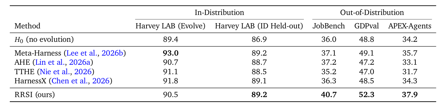
Only the agentic domain has per-opponent numbers; coding and engineering have only “the average of the four opponents” in Figure 1(b) and (d). What the columns mean: Harvey LAB (Evolve) is the 120 tasks used for evolution, Harvey LAB (ID Held-out) is the 40 tasks of the same benchmark that were not used, and JobBench, GDPval and APEX-Agents are three benchmarks never seen at all. The three OOD scores mean different things (weighted rubric, win rate, task success rate), so the OOD average is only a convenient summary with no single meaning.
The table below is a comparison computed from Table 1, with each number being the gain over the unevolved . The OOD-average column is my own calculation; the paper gives the and RRSI averages only in Table 2 and Figure 1:
| Method | Evolve gain | ID held-out gain | OOD average | OOD average gain |
|---|---|---|---|---|
| (unevolved) | - | - | 39.7 | - |
| Meta-Harness | +3.6 | +2.3 | 40.6 | +0.9 |
| HarnessX | +2.4 | +2.2 | 39.7 | 0.0 |
| AHE | +1.3 | +1.8 | 39.2 | |
| TTHE | +1.7 | +1.6 | 38.0 | |
| RRSI | +1.1 | +2.3 | 43.6 | +3.9 |
The table says three things. On the evolution tasks, RRSI gains the least (+1.1) and Meta-Harness the most (+3.6). On tasks of the same benchmark that were not used, everyone is about the same, with RRSI and Meta-Harness tied for highest (+2.3). The gap appears on benchmarks never seen: RRSI gains +3.9 on average, 3.0 points above the strongest opponent Meta-Harness, while two other opponents fall below . RRSI is first on all three benchmarks, ahead of each one’s strongest opponent by 3.5 (JobBench), 3.2 (GDPval) and 2.2 (APEX-Agents) points. In other words, the more a method gains during evolution, the less stable it is after switching tasks, and RRSI deliberately trades evolve score for transferability.
Doubts and limitations:
- The paper does not say how many times each method’s evolution was re-run, and there are no standard deviations. Inference: being first on all three benchmarks, with margins larger than the gaps among the opponents themselves (best 40.6 versus worst 38.0), looks less like plain luck, but this is not a statistical test.
- “OOD” here is only a change of tasks within the same domain: evolving on Harvey LAB (legal) and testing on other workplace-task benchmarks. There is no cross-domain test, such as taking a harness evolved on coding to workspace tasks.
- The opponents were re-run by the authors, and the paper does not say whether the opponents were tuned, or whether their proposer is the same model.
6.3 Main Result: The Three Domains
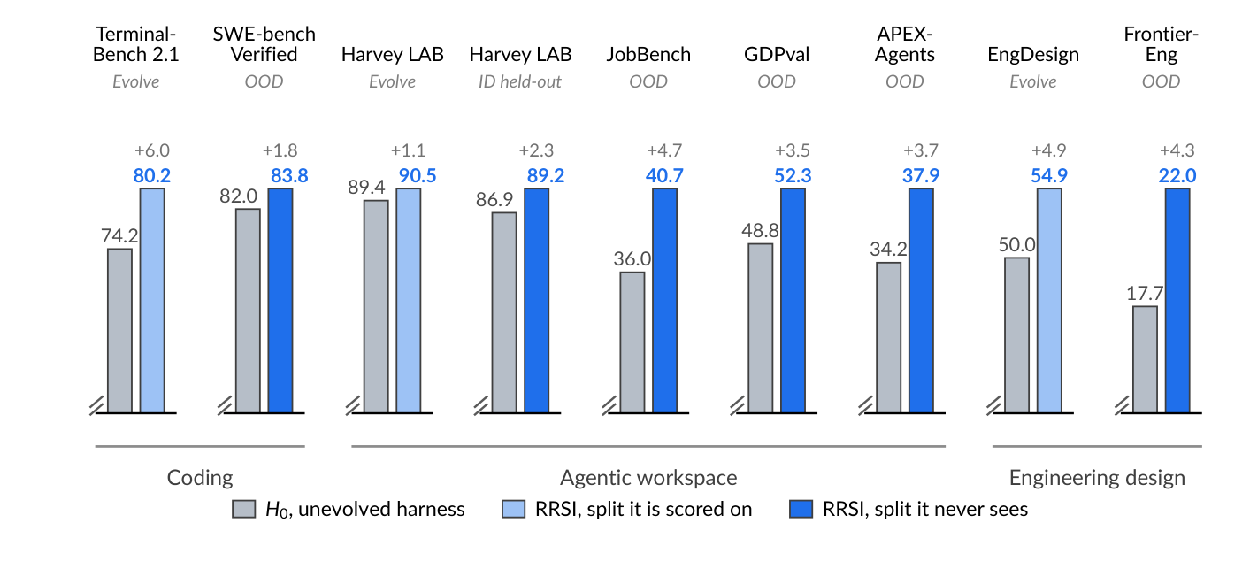
Figure 3’s numbers, tabulated:
| Domain | Evolution benchmark | Gain | Benchmark never seen | Gain |
|---|---|---|---|---|
| coding | Terminal-Bench 2.1: 74.2 to 80.2 | +6.0 | SWE-bench Verified: 82.0 to 83.8 | +1.8 |
| agentic | Harvey LAB: 89.4 to 90.5 | +1.1 | JobBench, GDPval, APEX-Agents | +3.5 to +4.7 |
| engineering | EngDesign: 50.0 to 54.9 | +4.9 | Frontier-Eng: 17.7 to 22.0 | +4.3 |
- Coding’s OOD gain is small: SWE-bench’s +1.8 points is about the size of coding’s noise band of 1.7 points. They are different benchmarks and cannot be compared as a test, but this gain is hard to tell apart from noise (inference).
- Frontier-Eng’s +4.3 comes from a very small base: 4.3% is roughly the weight of 1.6 to 2 gold medals (taking 38 or 47 as the denominator), so the “24.3% relative gain” in the paper’s abstract sounds large but underneath is a difference of a few tasks.
6.4 Ablation: What Regularization Itself Contributes

This is the only place in the paper where the contribution of regularization itself can be seen. The cleanest comparison is “no regularization at all” against “RRSI” (computed from Table 2 below; the paper does not list it directly):
| Comparison | Evolve | ID held-out | OOD average | Tokens/trial |
|---|---|---|---|---|
| to Unregularized (evolution alone) | +3.4 | +2.0 | +0.6 | 1.56M to 3.80M (+144%) |
| Unregularized to RRSI (the regularizers’ contribution) | +0.3 | +3.3 | 3.80M to 2.42M () | |
| to RRSI (total gain) | +1.1 | +2.3 | +3.9 | 1.56M to 2.42M (+55%) |
Evolution with no regularization gains the most on the evolve score, but barely improves on unseen tasks (only +0.6) and uses more than twice the tokens. With regularization added, the evolve score is 2.3 points lower, OOD is 3.3 points higher, tokens drop by a third, and ID held-out differs by only 0.3.
Removing the regularizers one group at a time gives these four rows:
| Variant | Evolve | ID held-out | OOD average | Tokens/trial |
|---|---|---|---|---|
| RRSI (everything) | 90.5 | 89.2 | 43.6 | 2.42M |
| Without the proposal side (A, B, C) | 90.7 | 88.8 | 41.9 | 2.69M |
| Without the acceptance side (D, E, F) | 91.5 | 88.7 | 41.0 | 3.59M |
| Everything removed | 92.8 | 88.9 | 40.3 | 3.80M |
The pattern is tidy: the more regularization removed, the higher the evolve score (90.5, 90.7, 91.5, 92.8) and the lower the OOD (43.6, 41.9, 41.0, 40.3). This is exactly the tradeoff the paper wants to demonstrate.
Doubts and limitations:
- Every row has just one number and no standard deviation, so how stable the 3.3-point OOD gap is cannot be judged.
- The ablation was done in only one domain, agentic, and not in coding or engineering.
- There is still no ablation of any single component, only two large groups. The paper is inconsistent about which group G belongs to, and Table 2 does not say.
- “Unregularized” does not say whether it includes the analyst feedback and history records, only that A through G were removed. The paper’s abstract says “30% fewer tokens”, while I calculate 36% fewer in this comparison, and the paper does not say what the 30% was compared against.
- The numbers in the paper’s abstract are the best-looking picks: “up to 14.1 points gain” is the gain of the weaker model on the evolution tasks in Table 3, “up to 4.7 points on OOD” is the best of the three benchmarks, and “22.9% above existing methods” is Frontier-Eng’s 17.9 to 22.0 (Figure 1(d)), where the base is small and the relative percentage is inflated. The 17.9 base here differs slightly from Figure 3’s 17.7, and the paper does not explain the difference.
6.5 Other Experiments: Changing the Model, the Cost and the Grading
These experiments are supporting evidence, not the core of the proof, so only the results and a one-line reservation are given.

Table 3 checks whether the effect persists when re-evolving with a model from a different family. The results:
| Policy | Terminal-Bench 2.1 (evolve) | SWE-bench Verified (OOD) |
|---|---|---|
| Claude Opus 4.8 | 74.2 to 80.2 (+6.0) | 82.0 to 83.8 (+1.8) |
| Gemini 3.5 Flash | 64.6 to 78.7 (+14.1) | 76.8 to 79.0 (+2.2) |
Doubt: the “14.1” in the paper’s abstract is exactly this row (evolution tasks, weaker model). SWE-bench gains are only about +2, the same order as the coding noise band. Only two models were tested, with no standard deviation.

Table 4 looks at whether the evolved harness still helps when moved to a weaker model that did not take part in evolution. Gemini 3.1 Flash Lite goes from 11.2 to 14.6 (+3.4). The paper writes a relative gain of 30.4%, but the absolute gain is only +3.4, about a quarter of the +14.1 on the evolution model. Doubts: it tests the same tasks used for evolution, so it only validates changing the model, not changing the tasks. Flash Lite and the Flash used for evolution are both Gemini, not a cross-family test. There is only one weak model, and it was only tested in the weaker direction.
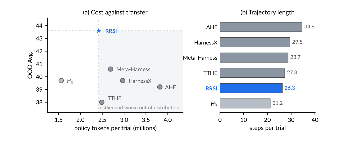
Figure 4 says RRSI spends the least of all the evolution methods. RRSI uses 2.42M tokens and 26.3 steps per trial, while the opponents use 27.3 to 34.6 steps. AHE is the most expensive at 3.82M tokens (58% more) and still has 4.4 points lower OOD. Doubt: RRSI is still 55% more expensive than the unevolved (1.56M, 21.2 steps). TTHE and RRSI are close, and the advantage is mostly pulled apart by AHE. This measures only the cost of running the final harness once, and the paper does not report what the evolution process itself (20 rounds, several candidates per round, three LLMs) costs.
Last is the deterministic grading in the second half of Section 4.2: EngDesign and Frontier-Eng are graded deterministically by simulators and the gains persist (+4.9, +4.3), used to show the gains are not from pandering to an LLM judge’s taste. Doubt: this only proves it for the engineering domain. One of JobBench’s judges is the same Opus 4.8 as the policy, and one of GDPval’s judges is also from the Claude family, and the paper does not discuss the possibility of judges favoring their own model family.
7 Overall Assessment
The value of this paper is in the reminder that “automatic harness evolution overfits easily and needs guardrails”, not in how novel the guardrails themselves are. My verdict is low research value and medium-to-high engineering reference value.
7.1 What It Really Achieves After Removing the Packaging
The cleanest comparison is the “evolution with no regularization at all” against “RRSI” computed in the ablation section: with the guardrails added, the evolution tasks lose 2.3 points (92.8 to 90.5), the unseen tasks gain 3.3 points (40.3 to 43.6), and tokens per trial drop from 3.80M to 2.42M, a third saved. This is the paper’s most solid evidence. The other numbers in the abstract are all the best-looking picks, and only this group is really stable, and only in the agentic domain.
7.2 Research Value and Engineering Value
Research value is low: the research contribution is close to “a good problem statement plus a set of sensible engineering rules”, with no new algorithm or theory. The paper also derives no generalization guarantee, and “regularizing the search trajectory” is a design framework plus an analogy whose effect is supported by experiments, not theory. Engineering reference value is medium-to-high: the rules are concrete and can be implemented from the description, and the design principles hold independently of this paper.
| Aspect | Strengths | Weaknesses |
|---|---|---|
| Research | Explains clearly that “harness evolution overfits” and points out three concrete behaviors. The risk of repeatedly scoring on the same tasks is a real problem in itself | Most components are combinations of common practices: pre-scoring review, a noise floor, trading cost for score, keeping a history (this is a judgement). L0, L1 and L2 are just names (Concept 3) |
| Research | Has a whole-group ablation whose direction matches the paper’s claim. Has supporting experiments changing the policy, the model and the grading | No single-component ablation, so we do not know which component really helps. No comparison has a standard deviation, and the cross-method comparison covers only one domain |
| Engineering | The rules are all concrete and can be implemented directly. Code and the complete round-by-round records are public (Appendix E says they are on the project website, including proposals, critic decisions, acceptance decisions and full diffs) | Some key hyperparameters are not explained and some are not listed (how was chosen, how was measured, guard thresholds, weights). The cost of evolution itself is not reported, only the final harness’s cost |
| Engineering | Each guardrail maps to one clear failure mode, which makes troubleshooting easier | The critic and proposer are the same LLM, so their blind spots may overlap (inference) |
7.3 The Three Biggest Doubts
- No variance. Every number is the result of one evolution, and the paper does not say how many times it was re-run. How stable the 3.3-point OOD gap is cannot be judged.
- “Generalization” is only a change of tasks within the same kind. There is no cross-domain test, such as taking a harness evolved on coding to workspace tasks.
- No component has evidence of its own. The paper’s core selling point is “this whole bundle of guardrails works”, not “this component works”.
7.4 What Is Worth Keeping, Ranked by Durability
| Durability | Content | Judgement |
|---|---|---|
| Medium | Explaining clearly that “automatic harness evolution overfits” and distilling three behaviors: fitting a specific benchmark, chasing noise, accumulating complexity | The problem statement itself has value and is the paper’s most real contribution |
| Medium-low | A full engineering recipe of guardrails (A through G plus the guard), supported by a whole-group ablation in agentic | Every component is a combination of common practices, and no single component has any evidence |
| Low | The specific numbers (OOD +3.3, 36% fewer tokens) and the L0 / L1 / L2 naming | The numbers are from one domain with no variance and will go stale with new models. The naming is only a metaphor and can be ignored |
In one sentence: this paper is close to a good problem statement plus a set of sensible engineering rules that were never validated piece by piece. What is truly durable are the general ideas in Concepts 1 to 4 and 6 of the extensions.
8 Extensions: Nine Concepts Worth Pulling Out
The nine sections below are the ideas that are easiest to get stuck on while reading this paper and easiest to forget. Concepts 1 to 4 and 6 are general ideas that hold independently of this paper. Concepts 5, 7, 8 and 9 are open questions the paper leaves behind, and they reference the method and formulas from the first half, so it is best to read the corresponding method sections first.
8.1 Concept 1: Why Repeatedly Deciding on the Same Data Manufactures Fake Progress
Start with the simplest scenario: you have 100 tasks to evaluate a system. Evaluate once and use that score as “the system’s level”, and it is an unbiased estimate with at most random noise. The problem is that you do not evaluate just once: you look at the result, change the system based on it, evaluate again on the same tasks, change it again, and so on.
The direction of the second modification was decided by the first evaluation’s result on these tasks, so the modification already carries “features of these tasks”. By the third evaluation, part of the score you measure is the result of “I tuned this for these tasks”, not real strength. These tasks are no longer independent test data. Statistically this is called adaptive data reuse, and the related research area is adaptive data analysis (Dwork et al. 2015 is a representative paper, which this paper cites to show that the problem exists, without deriving anything itself).
What follows is general statistical knowledge, not content from the paper. There are two amplifiers:
- Every score carries random noise, and every round is “pick the highest from a pile of candidates”. Taking a maximum systematically picks the one inflated by noise (see Concept 2). Take every candidate’s true effect as 0 and the noise standard deviation as : picking the best of 4 candidates gives an expected value of about , and picking the best of 100 scorings gives about . Nothing improved, yet it looks like progress, and the more you look, the bigger the fake progress.
- The bigger and more flexible the space, the easier it is to find modifications that “just happen to fit this set of tasks”. Harness evolution’s search space is “edit any source code”, a space of unusual expressiveness, so the paper calls it adaptive empirical optimization over an unusually expressive search space.
There is really only one remedy: the tasks used for evolution and the tasks used for the final check must be separate, and the check tasks must take no part in any decision, including tuning hyperparameters. This paper’s hyperparameters were chosen using only the evolve environment, without consulting held-out or OOD (Table 5’s caption).
The problematic way to write it is to evolve and check on the same tasks:
for t in range(T):
    candidates = propose(current, feedback(current, tasks))
    current = max(candidates + [current], key=lambda h: score(h, tasks))
final_score = score(current, tasks)   # this number was "seen" by the search, so it is inflated
The better way is to keep the check tasks out of every decision:
evolve_tasks, holdout_tasks = split(tasks)
for t in range(T):
    candidates = propose(current, feedback(current, evolve_tasks))
    current = max(candidates + [current], key=lambda h: score(h, evolve_tasks))
final_score = score(current, holdout_tasks)   # measured only once, at the end
RRSI does not manage “never reuse the same tasks during evolution” (it cannot, since the evolve set exists to be scored repeatedly). Instead it uses a set of guardrails to reduce the damage from reuse. The paper derives no generalization guarantee, and “regularizing the search trajectory” is a design framework plus an analogy.
This is also the most durable idea in this group: every “automatically improve, automatically evaluate” system (prompt optimization, skill evolution, agent evolution) has this structure.
Also, the evolution with no regularization at all is a valuable negative result in Table 2: it has the highest evolve score (92.8), yet gains only 0.6 on unseen tasks (39.7 to 40.3) and uses 144% more tokens. When evaluating any automatic evolution system, do not look only at its score on the evolution tasks: look at tasks that took no part in decisions, and look at cost too.
8.2 Concept 2: The Winner’s Curse
Pick the highest from a pile of scores that have some luck in them, and the one picked almost certainly has a score inflated by luck, so its true level is lower than the score you see.
Take an example: 4 candidates, all with exactly the same true strength of 90.0. But every scoring has random fluctuation (an LLM gives different results on each run, and each task is run only a few times), so the measured scores wobble around 90.0:
| Candidate | True strength | Score measured this time |
|---|---|---|
| A | 90.0 | 89.7 |
| B | 90.0 | 90.4 |
| C | 90.0 | 89.9 |
| D | 90.0 | 90.1 |
Pick the highest and B (90.4) is chosen. B looks like it gained 0.4 points, but B is really 90.0 like the others, and the extra 0.4 is purely luck this time. That 0.4 is the “curse”: you chose it because it was lucky, but when it is next re-scored the luck does not follow it, and the score falls back to around 90.0.
import random

def measure(true_score=90.0, noise=0.4):
    return random.gauss(true_score, noise)   # every scoring carries random noise

scores = [measure() for _ in range(4)]       # 4 candidates with identical true strength
best = max(scores)                           # the "winner"
Here best will on average be about 1.03 times noise above 90.0, and that gap is luck, not strength.
The term originally comes from auctions: the winning bidder tends to be the one who most optimistically values the item, and usually pays more than its true value. The “winner” wins partly because of luck, so what is won (that high score) cannot be taken at face value. The more candidates, the larger the inflation: picking the highest of 4 candidates inflates the expectation by about 1.03 noise standard deviations, and of 100 about 2.51.
How it relates to this paper:
- Every round RRSI “picks the highest score from a pile of candidates”, so every round has this problem.
- The selected candidate’s score is recorded as the historical best , and this inflated number then affects the later score-floor decisions (Concept 4).
- The earlier gates (critic, score floor, cost rule) filter out clearly problematic candidates, but the last step still picks the highest among survivors, so the winner’s curse is not eliminated, only reduced.
The practical rule: whenever a process has a step that “picks the highest from a pile of candidates”, assume that highest score is inflated and do not treat it as the true level.
8.3 Concept 3: Regularization, and What L0, L1 and L2 Each Do
With only training samples, a model that is too flexible will even memorize the noise in the data, giving a very low training error and doing badly on a new batch of data. Regularization adds a complexity penalty to the optimization objective:
- : the model’s parameters, which you can picture as a row of knobs.
- : the model’s prediction for the -th input . : the correct answer for the -th sample.
- : the error of a single prediction. times the sum averages the errors, which is the training error.
- : the complexity penalty, for example “how far the knobs are turned in total”.
- (greater than or equal to 0): the penalty strength. The larger it is, the more it prefers simple models.
Made-up numeric example: . Model A has a training error of 0.0 and complexity , for a total of . Model B has a training error of 0.5 and complexity , for a total of . The lower the total the better, so B is chosen: A memorizes the training data perfectly, but it is too complex and gets penalized.
Note the two key points: what is penalized is “the model’s own parameters ”, and where it acts is “the optimization objective”. This is “restricting the hypothesis space”, and the hypothesis space is the set of all possible models.
A norm is a way to “measure how large a vector is”. Let :
The first counts how many parameters are nonzero, the second sums the absolute values of all parameters, and the third sums the squares of all parameters. Made-up example: . L0 is 2 (two nonzero), L1 is , and the square of L2 is . Putting them into the penalty term gives three kinds of regularization:
| What takes | Name | Effect | Note |
|---|---|---|---|
| L0 norm | L0 regularization | Directly counts “how many knobs are on”, limiting the number of nonzero parameters | “Counting” cannot use gradient descent, so it is hard to optimize and rare in practice |
| L1 norm | Lasso (Least Absolute Shrinkage and Selection Operator) | Pushes unimportant parameters to exactly 0, giving a sparse model | Also selects variables |
| Square of the L2 norm | Ridge (ridge regression) | Shrinks all parameters together but rarely makes them exactly 0 | The most common in ML, and weight decay is essentially this |
Why does Lasso zero things out while Ridge does not? Look at the slope. Lowering a parameter from 0.1 to 0, L1’s penalty drops by 0.1, while L2’s penalty drops by only 0.1 squared, which is 0.01. The slope of is always 1, so it keeps pushing the parameter all the way to 0. The slope of is , and the closer to 0 the weaker the push, so it never gets there.
How this paper borrows these three names is really only a metaphor:
| The paper’s name | What RRSI actually does | How well it matches |
|---|---|---|
| L0: annealed edit budget (A) | A candidate bundles at most modifications, formally a cap on a count | Matches in form, but it is a hard cap, not a penalty term, and dropping the “L0” label loses no information |
| L1: structural pruning (G) | Components with no recent positive gain are listed as deletion targets | Only the intent of “sparsifying” is the same; the mechanism is closer to pruning in neural network compression |
| L2: complexity-aware acceptance (F) | Extra tokens must be offset by a score gain | A cost-benefit threshold with no squaring and no shrinkage, the weakest match |
The paper admits in Appendix C that this is a functional analogy, not optimizing any norm-penalized objective. So these terms do not make RRSI inherit L1’s sparsity or L2’s shrinkage, and when you see “L1-style” you only need to understand it as “cutting what contributes nothing”. Also, Figure 2 labels F as L1 and G as L0, which is inconsistent with the main text (A is L0, G is L1, F is L2). I judge it to be a slip (inference, not stated by the paper).
8.4 Concept 4: The Noise Band δ, the Score Floor, and a Stricter Version
A system scored repeatedly never gets exactly the same score each time (an LLM gives different results on each run, and each task is run only a finite number of times). Score the “completely unmodified version” several times, and the size of the natural wobble is the noise band . If a score difference is smaller than , you cannot tell whether it is a real difference or noise. The practice itself is very general: before evolving, score the unmodified version repeatedly, measure the size of the fluctuation, and only then decide what counts as progress.
scores = [evaluate(H0, tasks) for _ in range(R)]   # before evolving: re-evaluate the unmodified version
delta = spread(scores)                             # natural fluctuation size; you choose the statistic

lenient = score >= best_so_far - delta   # only blocks consecutive small regressions, lets lucky fake progress through (the paper's approach)
strict  = score >= best_so_far + delta   # blocks fake progress, but wrongly rejects unlucky real progress
The score floor (paper Eq. 5) is : a candidate’s score cannot be lower than the historical best by more than .
Why tie the floor to the historical best rather than the incumbent? To stop the search from walking downhill continuously. Made-up example, using coding’s and points:
| Round | Floor tied to the “incumbent” | Floor tied to the “historical best” (Eq. 5) |
|---|---|---|
| Start | Incumbent 74.2, floor 72.5 | , floor 72.5 |
| Round 1, candidate 72.6 | Passes. Incumbent becomes 72.6, floor drops to 70.9 | Passes. The floor is still 72.5 |
| Round 2, candidate 71.0 | Passes. Incumbent becomes 71.0, floor drops to 69.3 | Rejected (71.0 72.5) |
| Round 3, candidate 69.4 | Passes. Cumulative regression is already 4.8 points | Cannot happen |
Each step’s regression (1.6, 1.6, 1.6) is within , but accumulated it is a lot. Tied to the historical best, the floor only rises with the best and never falls, so over the whole evolution the score is at most below the best.
Eq. 5 sets only a lower bound and does not block “lucky fake progress”. The paper describes this component using noise chasing, but a candidate whose true level did not change and which merely measured 0.3 points higher this time passes Eq. 5 easily. To block this kind of fake progress, the statistically sensible approach is to also set an upper bound: require the candidate to beat the historical best by at least . The tradeoff between the two rules is below (made-up numbers, with and ):
| Situation | Lenient (the paper, ) | Strict () |
|---|---|---|
| True level equals the current one, but it measured 79.5 by luck this time | Passes. If it is the highest this round it will be selected, becoming fake progress | Does not pass (79.5 79.7), the fake progress is blocked |
| True level 1 point higher (real progress), but it measured 77.5 by bad luck this time | Passes, but since it is below it will not refresh | Does not pass (77.5 79.7), the real progress is wrongly rejected |
The lenient version’s cost is false positives (letting through fake progress propped up by noise), and the strict version’s cost is false negatives (blocking real progress that was unlucky). They solve different problems: the lenient one guards against consecutive small regressions and the strict one guards against fake progress, and the paper does only the former. My inference is that the paper may have feared setting the threshold too strict, so that over 20 rounds almost no candidate could pass and the search would get stuck, but this is only a guess, and the paper does not defend the choice.
Which to choose depends on which error you fear more: if the search budget is ample and fake progress is costly, choose strict. If the budget is tight and you fear the search stalling, choose lenient.
Two more limitations to remember: was measured on the original version, and the evolved version’s noise may not be the same. And records the measured score of the selected candidate, and the selected one is the highest, so itself may be inflated by luck (Concept 2). Later floors are then too high as well, and candidates of equal strength may be wrongly blocked.
8.5 Concept 5: What the Failure Feedback Is
is the write-up of “where the current harness fails” handed to the proposer each round. The paper says only who writes it and where it comes from, and not what it looks like. Three things the paper states explicitly:
| Content | Source |
|---|---|
| The current harness runs on the evolve set, produces trajectories (the complete record of a task run), and these are organized into | Section 2 |
| The one organizing it is a separate analyst LLM, the model being Claude Opus 4.8 | Section 4.1 |
| In the algorithm it is the Analyze(, ) step, which outputs | Algorithm 1, line 1 |
The flow is: runs on the evolve set and produces trajectories. The analyst LLM reads the trajectories and writes the failure feedback . is handed to the proposer as one of the conditions of the proposal distribution (Eq. 8).
What the paper does not explain: the format of (free text, a list, or structured fields), whether it carries per-task scores and failure reasons, whether the analyst reads all trajectories or a sample, and whether the proposer can also look at raw trajectories in addition to . Appendix B says the baseline Meta-Harness’s proposer can see execution traces, and whether RRSI has this access is not stated in the text.
There is also an inconsistency: Section 4.1 says the analyst produces “cross-round failure feedback”, but Appendix C.1 says is “feedback from the current round”. The difference between the two readings:
| Reading 1: current round only | Reading 2: cross-round aggregation | |
|---|---|---|
| Content of | Analyzes only ’s performance this round | Also synthesizes failure patterns from the past few rounds |
| Consequence | and the history have a clean division of labor: says the present and says the past | and overlap in function |
The paper’s text cannot settle which it is. What follows is my inference, which the paper does not state:
- is probably a summary of failure patterns. The clue is Engineering R2 in Table 6: the candidate added a recovery hint for the recurring tool error “workdir must be an existing directory”. To propose against it, the feedback most likely already organized “this error keeps recurring”.
- It cannot be the full raw records. Agentic evaluates 120 tasks × = 240 runs per round, and Table 2 shows consuming 1.56M policy tokens per run (possibly including context re-read at every step), so the whole batch far exceeds a context window. So the analyst must compress, and the paper does not write how.
- is the entry point for task-specific information into the search. Failure feedback inevitably mentions concrete tasks and concrete errors, and the proposer’s easiest fix is to hard-code those details into the harness, which is exactly what D blocks, and it also explains why the critic reads the code diff rather than just looking at scores.
The difference between and (component B):
| (component B) | ||
|---|---|---|
| What it records | Where the current harness fails | The outcome of every past modification |
| Who produces it | Organized by the analyst LLM | Recorded by code; who assigns the labels is not stated |
| Form of content | Not stated in the paper | A 7-tuple (see the section on B) |
8.6 Concept 6: The Annealed Budget Schedule: How the Formula Works and Where the Term Comes From
The annealed budget is a numeric schedule that is “loose early, tight late”, which is essentially a learning rate scheduler, except that what is scheduled is “the most modifications a candidate may bundle at once”.
Where the term comes from (general knowledge, not content from the paper):
- “Annealing” originally comes from metallurgy: heat metal and cool it slowly so its internal structure stabilizes.
- Entering optimization it became simulated annealing: a “temperature” schedule that falls over time, allowing large random moves early and only small adjustments late.
- Cosine annealing: the 2016 SGDR paper used the cosine shape for deep learning learning rate schedules, and it is now very common when training LLMs.
- All this paper borrows is the “loose early, tight late” shape, with no use of temperature or probabilistic acceptance.
The formula (paper Eq. 4, symbols in the section on A) breaks into four steps:
- is an angle that goes from 0 to as goes from 0 to , that is, from 0 degrees to 180 degrees.
- falls with it from 1 to .
- turns it into a coefficient falling from 1 to 0, with an S shape that is flat at the start, steep in the middle and flat again at the end, not a straight line.
- , that is, interpolate between the starting point and the ending point by the coefficient, and round up to an integer (because it counts “how many modifications”).
With coding’s settings (, , ), three points:
| Angle | Coefficient | |||
|---|---|---|---|---|
| 0 | 0 degrees | 1 | 1 | |
| 8 | 72 degrees | about 0.309 | about 0.6545 | |
| 19 | 171 degrees | about | about 0.006 |
Rounding brings two consequences (derived from the formula, not discussed in the paper). First, the coefficient only reaches 0 at , but one evolution runs only to , so the budget never reaches and stops at 2 at minimum. Second, after rounding the whole schedule has only three steps, 4, 3 and 2 (the full 20-round table is in the section on A). The cosine shape only decides in which round the steps switch, unlike a learning rate schedule: a learning rate is continuous, so the shape really affects training. Here the value is an integer, and cosine and a linear decrease give nearly the same result.
Behind this schedule is a more general design lesson: when several modifications are bundled in one candidate, they share the same measurement, so the records look like each one’s own contribution when it is only their combined contribution. So keep each change single and attributable where possible. When bundling is unavoidable, do not treat the shared score as each one’s own score. How to split credit among modifications when bundling is unavoidable is a separate topic that is not expanded here.
8.7 Concept 7: How to Push the Proposer to Explore
First be clear about which “amount of exploration” is meant:
| Quantity | How it is decided | Does it change during the run |
|---|---|---|
| : the most modifications each candidate may bundle | Determined by the formula in Eq. 4 | Only decreases (4 to 3 to 2) |
| : exploration slots reserved when stalled | A Table 5 hyperparameter, 1 in all three domains | Fixed, activated only when a stall is detected |
| The size of : the number of component categories not yet touched | The full set (9 categories) minus those touched | Only shrinks, starting at 9 |
- : Appendix D.1 says only that all hyperparameters were chosen using the evolve environment and operational considerations, with no sensitivity analysis, and the paper does not say why it is 1.
- : the full set is a hard-coded 9 categories, and the touched categories are cumulative (once touched, always counted), so only shrinks. Whether a component returns to after being pruned is not stated in the paper.
- The total number of candidates per round cannot be found as a concrete number in the paper, so what fraction of all candidates “reserving 1 slot” is cannot be judged.
“Forced exploration” is not actually forced. The paper’s wording is only reserved and redirect, and it writes no enforcement mechanism. What the paper actually provides:
- Check : whether the gain over the last rounds exceeded the noise band .
- Compute : the component categories not yet touched.
- Package them as as one of the proposer’s inputs (Eq. 8, Algorithm 1 lines 6 and 8).
- The proposer LLM generates candidates, and the paper does not say how it uses .
- Candidates go through the critic and selection as usual. No step checks whether the proposer complied (the critic blocks leakage, not lack of exploration).
Made-up example: suppose is written as a passage of text placed in the proposer’s prompt: “Gains in the last 3 rounds are within noise. Please propose at least 1 candidate that modifies one of these components not yet tried: skill, memory, subagent, client_tool.” Whether the proposer complies depends entirely on the LLM following the prompt. The paper’s text has two readings:
| Reading 1: just a sentence in the prompt | Reading 2: handled separately in code | |
|---|---|---|
| Meaning | The LLM decides for itself whether to comply | For example a dedicated proposal call that may only modify |
| Consequence | The exploration effect is not guaranteed and the proposer can ignore it | The exploration slot is certain to be produced |
The paper cannot settle which. Inference: Reading 1 is more likely, because Appendix C describes everything in the “input condition” language of .
The harder push toward exploration in the paper is on the selection side: the term in Eq. 17 gives a candidate that “tries a structural component that has never appeared in a winning modification” an extra bonus, making it easier to accept. This is the rule that truly favors new attempts, but with three limits: it is used only when the score falls inside the noise band. It works only for the four structural component categories client_tool, skill, memory and subagent. And its definition of “new” differs from C’s (C looks at “has it been measured”, the bonus looks at “has it won”). And the paper says the weight is listed in Table 5 when it is not, so how strong this bonus is cannot be known from the paper.
8.8 Concept 8: Where Do the Candidates the Critic Blocks Go
A candidate blocked by the critic before scoring has no score, and every entry in the history needs a score, so they are probably not in the history, and the proposer cannot see “which ideas were blocked for leakage”.
The order a candidate goes through (Section 3.3 and Appendix C.3 both say the critic runs before the full evaluation):
- The proposer proposes a candidate.
- The critic reads the code diff and decides whether it hard-codes task information. If blocked, it stops here and is never run on the evolve set.
- A candidate that passes is fully scored on the evolve set, giving and .
- It is written into the history .
The scores (, ) are produced only after step 3 finishes. A blocked candidate stops at step 2 and has never been executed, so it has no score. Each history record is a 7-tuple, with and required fields, which cannot be filled without a score. Just before writing out the record formula, Appendix C.2 has a half sentence “Ignoring candidates that fail before a valid measurement is obtained”, meaning candidates that fail before getting a valid measurement are set aside for now.
The consequence is that the proposer reads to adjust its proposals, and with blocked candidates absent from it, it does not know which ideas have been blocked before. Made-up example: in some round candidate W adds to the prompt “for Acme’s reports, use format YY” and is blocked by the critic. In the next round the proposer reads and finds no trace of W, may propose something similar again, and the critic blocks it again. The cost is a wasted proposal slot plus one critic call. Inference: it does not waste the evolve set’s scoring budget, because blocked candidates are not scored.
There is an uncertainty here. That half sentence is a notation made while writing the formula, and does not say “candidates blocked by the critic are definitely not in the record”. The paper’s text has two readings:
| Reading 1 | Reading 2 | |
|---|---|---|
| What “fail before a valid measurement” refers to | Includes candidates blocked by the critic | Refers only to execution failures and broken environments, not candidates blocked by the critic |
| Consequence | The proposer sees no record of leakage blocks and may propose them again | Records of blocks may reach the proposer through another channel (for example this round’s ) |
The paper’s text cannot settle which. Circumstantial evidence: Appendix E says the project website publishes the complete round-by-round records, including the critic’s decisions, so the critic’s decisions are recorded, but where they are recorded and whether the proposer reads them, the paper does not write.
Behind this is a general rule: what can be blocked before the incentive is obtained should not be handled after the incentive has been obtained. With the critic reviewing first, a blocked candidate never gets the high score that would make it look attractive, and later rounds are not misled by its high score. The cost is what was described above: a blocked candidate has no measurement and cannot be written into a record of “every modification with its score attached”.
if critic_flags(diff):
    reject(candidate)               # review first, so there is no score to favor it
else:
    score = evaluate(candidate)     # only candidates that pass review get scored
8.9 Concept 9: Two Questions About the In-Noise-Band Rule
The rule here is Eq. 17: when a candidate’s gain does not exceed the noise band , decides whether to keep it.
Question 1: why does coding set to 0? The paper gives no reason, only the result: coding’s , so a score gain inside the noise band cannot by itself let a candidate pass, and it must rely on saving cost or trying a new structure. Agentic and engineering use a positive , and the paper does not explain why the three domains differ.
Inference (the paper does not say this): the purpose of this rule is “not to treat small score fluctuations as sufficient evidence” (Appendix C.3), and takes this principle to the limit, so score changes inside the noise band count for nothing at all. But this inference has a hole: coding’s is 0.017 and engineering’s is 0.020, larger than coding’s, yet engineering uses a positive . So “ is large, so do not trust the score” cannot explain the difference across the three domains, and I cannot find a consistent reason.
Question 2: is the rule meant to give small-gain modifications a chance to be accepted? Only half right.
| Claim | Judgement | |
|---|---|---|
| The purpose the paper states | Avoid treating small score fluctuations as sufficient evidence | The purpose is defensive, not opening the door for small gains |
| This rule’s role | Candidates inside the noise band are not bound by Eq. 7’s cost cap and need another rule to decide whether to keep them | It handles the gray zone of “cannot tell real progress from noise” |
| Can a small gain be accepted | Yes, but the route is not through the gain | The right part |
Candidates with a small gain really do have a chance of being accepted, but in coding the reason they are accepted is “saves cost” or “tried a new structure”, and the score gain itself earns no points. Look at two made-up candidates (coding, both inside the noise band):
| Candidate | Score | Cost | Result |
|---|---|---|---|
| S | 1 more task | Saves 10% | Passes, because it saves cost (as long as ) |
| T | 1 more task | 26% more | Rejected |
The two candidates have the same score gain and different results, and the deciding factor is entirely cost. So in coding this rule is more like “a candidate inside the noise band is kept only if it is cheaper or newer”. In agentic and engineering, because is positive, small gains really do earn points.
The rule also leaves a design lesson: the two branches (gain above the noise band goes to Eq. 7, otherwise to Eq. 17) differ greatly in leniency on the two sides of the boundary, which is what creates the 3-task versus 4-task cliff above. When designing threshold rules, check whether the two sides of the boundary differ too much.
9 Conclusion
RRSI points out a real problem in automatic harness evolution: every round is scored on the same tasks, so the evolve score rises while the gain after switching tasks shrinks. It governs this with a whole bundle of guardrails, the proposal side (A, B, C) plus the selection side (D, E, F, G). In the agentic ablation, with the guardrails added the evolution tasks lose 2.3 points, OOD gains 3.3 points and tokens drop 36%.
My verdict is low research value and medium-to-high engineering reference value, because the paper’s own evidence is limited: no number has a variance, “generalization” is only a change of tasks within the same kind, and no component has its own ablation. What is more worth borrowing are the design principles: keep the tasks for evolution and for validation separate, measure the scoring noise before deciding what counts as progress, make cost something that must be paid for with score, keep a record of every modification, and, when evaluating an automatic evolution system, look at tasks that took no part in decisions and at cost, not only at its own score.