rStar Deep Dive: How MCTS & Mutual Reasoning Boost LLaMA2-7B Accuracy from 12% to 64% Without Fine-tuning

1 Introduction

In this article, I’d like to share an exciting paper born from the collaboration between Microsoft Research Asia and Harvard University: Mutual Reasoning Makes Smaller LLM Stronger Problem-Solvers (rStar). Published in August 2024, this paper has been successfully accepted as an ICLR 2025 Poster!

In the evolution of LLMs, it is commonly believed that to enhance the reasoning capabilities of Small Language Models (SLMs, e.g., LLaMA2-7B), we must rely on data distillation from powerful models (like GPT-4) for Supervised Fine-Tuning (SFT). However, this paper presents a disruptive perspective: Small models actually possess sufficient potential; they simply lack the correct “guided thinking” and “self-verification” mechanisms.

The authors propose an architecture named rStar, which combines MCTS (Monte Carlo Tree Search) with a unique Mutual Reasoning mechanism. Impressively, without any fine-tuning or reliance on GPT-4, simply through algorithmic enhancement at inference time, rStar boosted LLaMA2-7B’s accuracy on the GSM8K math dataset from 12.51% to 63.91%, even allowing Mistral-7B to surpass many models that underwent specialized fine-tuning.

Next, we will delve into how rStar unlocks the deep reasoning capabilities of small models by mimicking human thinking actions (Action Space) and conducting peer-like mutual checks (Discriminator).

2 The Problem rStar Aims to Solve

Broadly speaking:

How to significantly enhance the reasoning capabilities of small models (SLMs) without relying on stronger models (like GPT-4) for data distillation.

We can categorize the problems rStar aims to solve into three levels:

2.1 Macro Challenge: The Reasoning Bottleneck of Small Models & Reliance on “Teachers”

• Status Quo: Small parameter language models (SLMs, e.g., Mistral-7B, LLaMA2-7B) perform far worse than large models on complex reasoning tasks (such as GSM8K math problems). Even with Chain-of-Thought (CoT), accuracy remains limited (e.g., Mistral-7B sits at only 36.5%).
• Problem: The current mainstream method for improving SLM reasoning is Fine-tuning, but this typically relies on “stronger models” (like GPT-4) to generate high-quality synthetic data or for knowledge distillation.
• Goal: The paper hopes to break this dependency and achieve “Reasoning improvements without a superior teacher LLM”, meaning the model improves its capabilities through Inference-time self-play, without the need for additional training or external supervision.

2.2 Technical Challenge I: “Ineffective Exploration” in the Generation Phase

When models attempt self-improvement (e.g., using methods like RAP for tree search), they face the following difficulties:

• Search Space Traps: SLMs have limited capabilities. If simply asked to “generate the next step,” they often wander within a low-quality reasoning space. The paper mentions that even when LLaMA2-7B uses the RAP method to explore 32 rounds, only 24% of the trajectories are correct.
• Monotonous Action Space: When traditional MCTS is applied to LLMs, the actions are usually singular (e.g., “propose the next sub-question”). This limits the model’s ability to simulate diverse human reasoning processes (such as decomposing problems, rephrasing questions, one-step reasoning vs. multi-step reasoning, etc.).

2.3 Technical Challenge II: “Unreliable Verification” in the Validation Phase

Even if the model generates multiple reasoning paths, selecting the correct one is a major issue:

• Difficulty of Self-Verification: Research shows that SLMs struggle to accurately assess whether their generated answers are correct (Self-verification is hard). Models often cannot distinguish between high-quality and low-quality reasoning steps.
• Limitations of Majority Voting: Traditional Self-Consistency (SC) relies on “Majority Voting,” which assumes the model is right most of the time. However, on hard problems, SLMs might generate wrong answers the majority of the time, rendering majority voting ineffective.
• Cost of Reward Models: Training a specialized Reward Model (RM) brings us back to the problem of needing labeled data or external supervision, and it is prone to Overfitting specific tasks.

In summary:

The core pain point this paper addresses is:

Small models cannot think of good approaches during “Generation” and cannot distinguish right from wrong during “Checking.”

rStar attempts to solve these two problems by improving the MCTS Action Space (making generation more human-like) and introducing “Mutual Reasoning” (having another peer model verify).

3 The Method Proposed by rStar

The rStar method proposed in this paper can be summarized as:

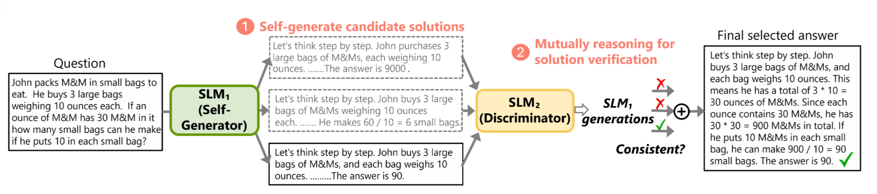
rStar is like making a small model play two roles: one role (the Generator) uses diverse thinking strategies mimicking humans (like decomposing problems, rephrasing) to generate solution paths; the other role (the Discriminator) acts like a classmate checking these paths through “fill-in-the-blank tests.” By verifying each other (Self-play), they significantly boost reasoning accuracy without retraining.

Understanding MCTS (Monte Carlo Tree Search) is key to grasping the technical details of this paper. The core backbone of rStar is built upon MCTS. Therefore, we will start with the basic concepts of MCTS, and then explain how rStar designs methods for each stage of MCTS.

3.1 Basic Concepts of MCTS (Four Stages)

MCTS is a heuristic search algorithm that first shone in board games like Go (e.g., AlphaGo). Its core idea is:

Since there are too many possible paths, I can’t calculate them all. So, I use “random simulations” to estimate win rates, focusing computational resources on the “most promising” paths.

In the rStar paper, MCTS is used to help the Generator create reasoning steps. The Root of a tree is the problem, Nodes are intermediate reasoning steps, and Edges are the actions taken.

One Iteration of MCTS includes the following four standard stages:

1. Selection:

   • What: Start from the root and move down the tree until reaching a node that hasn’t been fully expanded (Leaf node).
   • How: This step isn’t random; it uses a formula (usually UCT, Upper Confidence Bound for Trees). This formula balances two things:
     • Exploitation: Take the path that currently looks to have the highest score/win rate.
     • Exploration: Take the path rarely traveled, as better answers might hide there.
   • Significance: Ensures we focus on the current best solution while not giving up on exploring unknown possibilities.

2. Expansion:

   • What: After “Selection” reaches a leaf node, if this node can be further deduced, we create one or more new Child Nodes.
   • Significance: In rStar, this represents the model taking a new reasoning action (like decomposing the problem, generating the next step) based on the current reasoning state, growing new reasoning steps.

3. Simulation (Rollout):

   • What: Start from the newly expanded node and quickly run to the end until the game is over or a complete answer is generated. This usually uses a simpler or random strategy (Default Policy).
   • Significance: This is like a “trial run.” Since we only generated half the reasoning steps and don’t know if they are right, we simply let the model quickly finish the remaining steps to see if a reasonable answer can be reached.

4. Backpropagation:

   • What: Based on the result of the “Simulation” (e.g., whether the final answer passed a check, or the Reward score obtained), pass this score all the way back to all parent nodes passed along the path.
   • Significance: Updates the statistics (Visit count $N$ and Value $Q$) for nodes on this path. If this simulation was successful, the score of nodes on this path increases, making them more likely to be selected in the next “Selection” phase.

3.2 The “Selection” Process in rStar

rStar doesn’t design anything specific for Selection, mainly following the original MCTS approach:

1. Start from Root: Begin at the question.
2. Face the Fork: Assume the current node is expanded, having generated several candidate Child Nodes ($s_1, s_2, s_3...$).
3. Score: Calculate the UCT score for each candidate Child Node.
4. Pick: Select the Child Node with the highest UCT score and move there.
5. Repeat: Continue steps 2-4 at the new Node until a “Leaf Node” is encountered (a node that hasn’t generated subsequent steps yet).

Once a leaf node is reached, the Selection phase ends, and the Expansion phase begins.

3.2.1 UCT (Upper Confidence Bounds for Trees)

In the Selection phase, how is the UCT score calculated? Let’s look directly at the formula in Section 3.2 (Solution Generation with MCTS Rollout) of the paper:

This formula determines which step MCTS should pick when facing multiple possible next steps (Child Nodes) during the Selection phase. It consists of two parts: Exploitation and Exploration.

3.2.1.1 Part 1: Exploitation — Picking “High-Performing Stocks”

• Meaning: This is the average win rate (average reward) of node $s$.

• $Q(s, a)$: The total accumulated score of the node.

  Meaning of Q(s, a)

  So, the precise meaning of \(Q(s, a)\) is:
  
  **"The total accumulated reward value of this specific reasoning step \(s\) (generated by action \(a\))."**
  
  *   **Scenario Simulation:** Suppose you are at "Step 1" and considering "Step 2 (Plan A)".
  *   Here \(s\) is "Step 2 (Plan A)".
  *   \(a\) is the action that produced Plan A (e.g., "Propose a sub-question").
  *   \(Q(s, a)\) is the total score we historically judged as helpful to solving the problem after passing through this node \(s\).
  

• $N(s, a)$: The number of times this node has been visited.

• Intuition: If we have walked this reasoning step 10 times before, and 9 times it led to the correct answer, its average score will be high. This term encourages the model to follow paths proven to be good by past experience.

3.2.1.2 Part 2: Exploration — Giving “Potential Stocks” a Chance

• Meaning: This gives bonus points to less traveled paths (Exploration Bonus).
• $N_{parent}(s)$: The total number of times the parent node (current location) has been visited.
• $N(s, a)$: The number of times the child node $s$ (the candidate we are evaluating) has been visited.
• Mathematical Mechanism:
  • Denominator is $N(s, a)$: If we have visited node $s$ many times, the denominator gets large, and this value becomes small (exploration bonus drops).
  • Numerator is $\ln N_{parent}(s)$: As we pass through the parent node more often, if a certain child node $s$’s visit count $N(s, a)$ hasn’t increased (remains 0 or very small), this value becomes very large.
• $c$ (Constant): This is a hyperparameter to adjust the weight of exploration. The larger $c$ is, the more the model likes to try fresh paths.
• Intuition: This term says: “Hey! Although the average score of that path (node $s$) over there might not be the highest, or is 0, that’s because we haven’t really walked it yet! Give it a chance!”

3.3 The “Expansion” Process in rStar

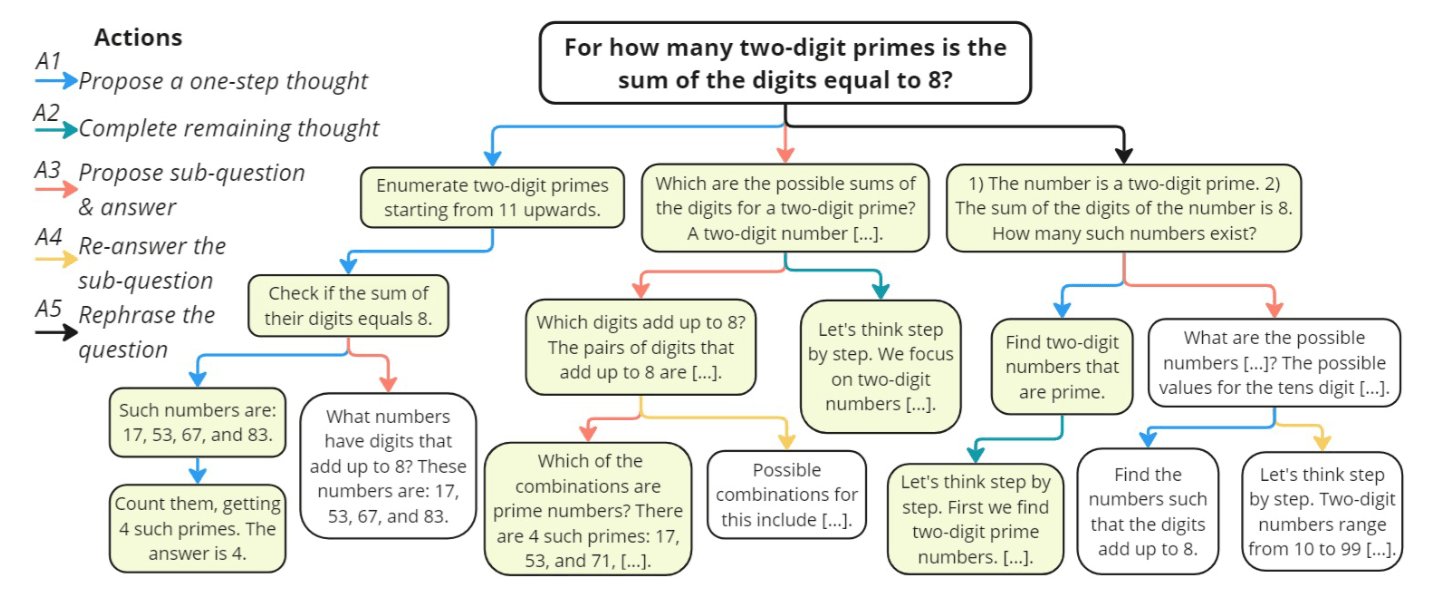
This is one of the most brilliant innovations of this paper! Traditional MCTS often only uses one way to “expand” (e.g., always asking “What is the next step?”). But rStar observed that human thinking is very flexible when solving hard problems.

In the Expansion phase, when MCTS reaches a leaf node (current reasoning state), it chooses one of 5 Actions mimicking human reasoning to execute, generating a new child node (new reasoning content).

I categorize these 5 Actions into three main groups: Linear Reasoning, Decomposition & Refinement, and Reformulation.

3.3.1 Category 1: Linear Reasoning

These actions are most like standard Chain-of-Thought (CoT), suitable for handling logical flows that are relatively smooth.

3.3.1.1 Action 1 ($A_1$): Propose a one-step thought

• What: Based on the current context, generate only the reasoning for “this step,” without rushing to write out the rest.
• Why: To avoid CoT’s “snowballing errors.” Standard CoT writes everything in one go; if the middle is wrong, the end is wrong.
• MCTS View: Expands a child node containing only the “next sentence.”

3.3.1.2 Action 2 ($A_2$): Propose the remaining thought steps

• What: Based on the current state, write out all remaining reasoning steps in one breath until the answer is reached.
• Why: This mimics human “fast thinking.” If the remaining problem has become simple, or the model is confident, there’s no need to drag it out step-by-step; rushing to the finish line is more efficient.
• MCTS View: Expands a child node containing the full subsequent path (usually leading directly to a terminal node).

3.3.2 Category 2: Decomposition & Refinement

These actions are specifically designed to tackle complex, error-prone problems, inspired by “Least-to-Most Prompting.”

3.3.2.1 Action 3 ($A_3$): Propose next sub-question along with its answer

• What: The model doesn’t solve the original problem directly but asks itself: “To solve this big problem, which small problem do I need to solve first?” and then answers this small problem.
• Why: Complex problems (like multi-step math questions) are easy to get wrong if solved directly. Breaking them into sub-questions lowers the difficulty.
• MCTS View: Expands a node containing a “Q: Sub-question… A: Sub-answer…” structure.

3.3.2.2 Action 4 ($A_4$): Answer the sub-question again

• Constraint: This action can only be used after $A_3$.
• What: Target the sub-question just proposed by $A_3$ and answer it again. But this time, force the model to use Few-shot CoT to answer in detail.
• Why: Sometimes $A_3$ identifies the right question but answers it sloppily or incorrectly. $A_4$ acts like a “checking mechanism” or a “more serious solving mode” to ensure this key sub-step is calculated correctly.
• MCTS View: This is a correction or reinforcement of the previous node.

3.3.3 Category 3: Reformulation

This action solves issues of “misinterpreting the question” or “tunnel vision.”

3.3.3.1 Action 5 ($A_5$): Rephrase the question/sub-question

• Constraint: Usually used after the Root (original question) or after sub-questions (mainly targeting the question text).
• What: Re-list the conditions in the question, or paraphrase it to make the question clearer.
• Why: Often models make mistakes because they miss a hidden condition in the question (like “positive integer”, “does not contain”, etc.). This action simulates a human saying when stuck: “Wait, let me re-read the question and list the known conditions…”
• MCTS View: The expanded node is not a reasoning step but a “clearer problem description,” and subsequent reasoning will be based on this new description.

3.3.4 Which Action to Choose Each Time?

In high-level systems like AlphaGo, there is usually a Policy Network to predict the probability of each action (Prior Probability).

However, in rStar, to remain lightweight and applicable to various SLMs, it does not train an additional Policy Network to decide which Action to pick. Instead, it uses “Rule-based Constraints” paired with an “Exploration First” mechanism. We can imagine it as a checklist with rules.

Specifically, the logic for deciding the Expansion action has two layers:

3.3.4.1 Layer 1 Filter: Hard Constraints

Not all 5 Actions can be used at any time; they must fit the current “context logic.” The paper clearly defines dependencies:

• $A_4$ (Answer sub-question again): Can only be used after $A_3$ (Propose sub-question).
  • Logic: You must have a sub-question first to “re-answer” it.
• $A_5$ (Rephrase): Can only be used after Root (original question) (or after sub-questions in some settings, but primarily for the prompt).
  • Logic: Usually needed only when the question is hard to understand or conditions are complex.
• $A_1, A_2, A_3$: These are more general actions, available in most Intermediate States.

3.3.4.2 Layer 2 Decision: UCT’s “Unexplored Priority” Mechanism

This returns to the core feature of MCTS. When Selection picks a node and prepares for Expansion:

• Initial State: For all Action types that haven’t been tried yet (the legal ones), their visit count $N$ is 0.
• Mathematical Result: According to the UCT formula, the denominator is 0 (or extremely small), causing the calculated value to be infinite.
• Decision: MCTS forces the model to try those Action types that “haven’t been tried yet”.

In other words, rStar’s strategy is “Rain or Shine (Even Distribution)”: It doesn’t prejudge which action is good but tends to try every legal action type once. If $A_1$ hasn’t been done on this node, do $A_1$; next time if $A_1$ is done, try $A_3$.

3.3.4.3 Supplement: Quantity Limit (Quota)

To prevent the search tree from becoming infinitely wide, the paper mentions an important limit in Section 4.1 (Implementation Details):

• $A_1$ (One-step) & $A_3$ (Sub-question): These two actions have high variance, allowing up to 5 different child nodes under the same node (by sampling different content).
• Other Actions ($A_2, A_4, A_5$): Default limit is 1.

3.3.4.4 Summary

So in the Expansion phase, the flow to decide the Action is:

1. List: List all legal Action types based on the current node state (remove illogical ones).
2. Check Quota: Check which Action types haven’t reached the generation limit.
3. Random/Round-Robin: Pick one from the remaining legal options (usually random or sequential) and let the LLM execute generation.

Conclusion: rStar doesn’t rely on the model to “judge” what move is best at the moment. Instead, it uses MCTS characteristics to force the model to try various moves over multiple Rollouts, and finally, the Reward mechanism tells the model which move was most effective.

3.4 The “Simulation” Process in rStar

Suppose we are now standing on a Child Node (call it $s_1$). This node was just generated via Action $A_1$ (Propose a one-step thought), so it currently only contains the “first step” of reasoning (e.g., “Step 1: First calculate how many apples there were…”), without a final answer.

If we stop here, we have no idea if this step is good. The purpose of Simulation (also called Rollout) is to evaluate whether this node ($s_1$) can lead to a correct ending by “fast-forwarding into the future.”

Here are the detailed steps for the Simulation phase in the rStar paper:

3.4.1 Default Policy Rollout

At this stage, MCTS switches to a simpler, faster mode (Default Policy).

• Input: Question + content of current node $s_1$.
• Instruction: Tell the LLM: “Based on the written Step 1, complete all remaining reasoning steps until the answer is calculated.”
• Action: Usually, complex actions like $A_3, A_4, A_5$ are not used here. Instead, it’s logic similar to Action $A_2$ (Propose remaining steps), letting the model generate to the end in one go.

3.4.2 Terminal State

After the LLM executes the instruction, it generates a Full Trajectory:

At this point, we have a final answer (e.g., “The answer is 42”).

3.4.3 Reward Calculation — The Key Scoring Standard

Now that we have a final answer, how do we score $s_1$ (calculate $Q$ value)?

The paper faced a major challenge: This is an inference task, so there is no Ground Truth to compare against. Therefore, rStar uses Self-Consistency Majority Voting Estimation.

In the Implementation Details of Section 4.1 Experiment Setup, the paper mentions “In the trajectory self-generation stage, we augment each target SLM with our MCTS, performing 32 rollouts.” This means the 4-stage MCTS process (Selection -> Expansion -> Simulation -> Backpropagation) runs 32 times. Each time yields a Full Trajectory and a Final Answer, resulting in a total of 32 Full Trajectories and Final Answers.

Thus, rStar compares the final answer obtained from each Simulation with the current pool of answers in MCTS (up to 32) to calculate the Reward:

1. Answer Pool: During the search process of the entire MCTS tree, we generate many paths and obtain many answers.
2. Self-Consistency Majority Voting: We check which answer appears most frequently. Suppose “42” appears most often among all attempts; we tentatively consider “42” to be the correct answer.
3. Reward:
   • If the answer from this Simulation is “42” (consistent with mainstream opinion), this simulation gets a High Score (Reward = 1).
   • If it is “15” (minority opinion), it gets a Low Score (Reward = 0).

In the early stages of MCTS (first few rounds), the answer pool is small, so this score might not be accurate. But as the number of Rollouts increases (the paper sets it to 32), the “correct answer” usually emerges due to probability advantages, and the scoring becomes more accurate.

3.5 The “Backpropagation” Process in rStar

If Selection is “Decision,” Expansion is “Action,” and Simulation is “Evaluation,” then Backpropagation is “Learning and Induction.” This is the key moment when MCTS truly gets smarter.

In the rStar paper, the implementation of Backpropagation is very intuitive, but there is a key design choice made to adapt to SLMs.

I break it down into three parts:

3.5.1 Core Task: Update What?

When Simulation ends, we get a Reward (let’s call it $R$). Now, we need to go back along the path we just walked (from the current Leaf Node all the way to Root Node) and update two statistics for every node on the path:

1. $N(s, a)$ (Visited Count):
   • Tell this node: “Hey, we passed through you again!”
   • Update: $N \leftarrow N + 1$
2. $Q(s, a)$ (Total Reward Value):
   • Tell this node: “After passing you this time, we got a result of $R$ points, put it on the ledger!”
   • Update: $Q \leftarrow Q + R$

3.5.2 rStar’s Key Design: Outcome-based Reward

This is a highlight of the paper. Many advanced MCTS methods (like AlphaGo) or other Reasoning methods (like RAP) try to score every intermediate step (Intermediate Reward).

But in rStar, the authors deliberately avoided scoring intermediate steps.

• Why? Because SLMs are weak; letting them evaluate “is this reasoning step good” (Self-rewarding) is usually inaccurate, sometimes no better than guessing (proven in the paper’s Appendix).
• How? rStar adopts a Sparse Reward strategy.
  • The “intrinsic value” of intermediate nodes is set to 0.
  • Their value depends entirely on the result of the final Simulation.

Specific Operation:

Suppose our generated path is: Root (Question) $\rightarrow$ Node A (Step 1) $\rightarrow$ Node B (Step 2) $\rightarrow$ [Simulation] $\rightarrow$ Final Answer

Assume Simulation gives a Reward $R = 0.8$ based on majority voting.

Backpropagation Update:

1. Update Node B:
   • $N_B \leftarrow N_B + 1$
   • $Q_B \leftarrow Q_B + 0.8$
2. Update Node A:
   • $N_A \leftarrow N_A + 1$
   • $Q_A \leftarrow Q_A + 0.8$
3. Update Root:
   • $N_{root} \leftarrow N_{root} + 1$
   • $Q_{root} \leftarrow Q_{root} + 0.8$

Significance: This implies that Node A and Node B share equal credit for this “good result.” This is a simplified but effective method of Credit Assignment.

3.5.3 Connection with UCT Formula

After this update, the data of the whole tree changes.

• Since $N$ increased, the Exploration term value for nodes on this path in the next Selection phase will decrease (denominator gets bigger).
• Since $Q$ increased (assuming $R$ is positive), the Exploitation term (average win rate $Q/N$) of this path might increase.

This forms a closed loop:

• If the result is good ($R=1.0$) $\rightarrow$ $Q$ increases significantly $\rightarrow$ Average score rises $\rightarrow$ More likely to be selected next time (Exploitation).
• If the result is bad ($R=0.0$) $\rightarrow$ $Q$ stays same but $N$ increases $\rightarrow$ Average score is dragged down $\rightarrow$ Might try other paths next time (Exploration).

3.6 rStar’s Mutual Reasoning for Final Answer

After finishing 32 Rollouts (Selection -> Expansion -> Simulation -> Backpropagation), we currently have 32 Full Trajectories and Final Answers. The next question is: How to decide the Final Answer?

So, rStar introduces the second stage: Mutual Reasoning and Discriminator. These 32 Trajectories go through a “strict filtering and verification” process:

3.6.1 Discriminator

• Who? Another SLM of comparable capability, or even the same model playing a different role.
• Task: Its job is not to directly score these 32 paths (e.g., “I give this 80 points”), because small models are bad at scoring.
• Method: Its job is a “Fill-in-the-blank Test.”

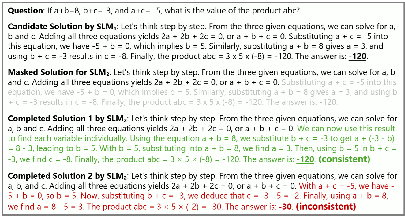
3.6.2 Mask-and-Complete

For each of these 32 Trajectories (let’s call it $t$), the system performs the following:

1. Masking:

   • Suppose a Trajectory $t$ has 5 steps total ($s_1, s_2, s_3, s_4, s_5$).
   • The system randomly selects a cut point (the paper mentions keeping the first 20% to 80% of steps).
   • For example, keep the first 3 steps ($s_1, s_2, s_3$) and Mask (hide) the rest ($s_4, s_5$).

2. Completion:

   • Feed the question and the kept first half ($s_1, s_2, s_3$) to the Discriminator.
   • Instruction: “Based on the previous steps, please complete the remaining reasoning steps and calculate the answer.”
   • The Discriminator generates a new ending and a new answer (noted as $\hat{A}$).

3.6.3 Mutual Consistency Check

Now we have two answers:

• Original Answer ($A$): From the full Trajectory generated by the Generator.
• Rewritten Answer ($\hat{A}$): Result from the Discriminator completing the first half.

Judgment Standard:

• If $A == \hat{A}$: Congratulations! This path is considered Mutually Consistent. This means the logic of this path is robust; even another model seeing half of it can deduce the same result. The credibility of this path increases significantly.
• If $A \neq \hat{A}$: Alert! This path might have logical jumps or luck factors, causing another model to fail to continue it or reach a different result.

3.6.4 Final Selection

Through Mutual Reasoning and the Discriminator, we can filter the 32 Trajectories generated. Based on the remaining Trajectories, we pick the unique “King” as the final response.

We calculate a score for the remaining Trajectories using the following formula, then pick the one with the highest score:

3.6.4.1 MCTS Reward

• Source: Data from the MCTS Search Tree (Generator).
• What it is: The $Q$ value (or normalized $Q$ value) of the terminal node corresponding to that Trajectory in MCTS.
• Significance: “How is the quality of this specific reasoning path?”
  • During MCTS, if this path ($t$) was visited multiple times and led to high-score answers each time, its $Q$ value will be high.
  • This implies the Generator thinks: “Following these steps, the logic is very smooth and stable.”

3.6.4.2 Confidence Score

• Source: Statistics from the Answer Pool of 32 Rollouts.
• What it is: The frequency of “that answer” appearing in all 32 attempts (i.e., Self-Consistency Majority Voting probability).
• Significance: “How credible is the final answer?”
  • This is irrelevant to the path, only looking at the result.
  • Example: If “42” was calculated 28 out of 32 times, the Confidence Score for “42” is $28/32 = 0.875$.

3.6.4.3 Why Multiply?

Suppose we have two Trajectories verified by the Discriminator (call them A and B), both yielding the correct answer “42”. Which one should we output as the “detailed solution”?

• Trajectory A:

  • A common, stable path (MCTS walked here often).
  • $Q$ Value (Reward) = 0.9 (High path quality)
  • Answer “42” Confidence = 0.875 (Answer is popular)
  • Final Score = $0.9 \times 0.875 = \mathbf{0.7875}$

• Trajectory B:

  • A rare path (MCTS rarely walked here, or it occasionally led to errors), but got it right this time and passed the Discriminator.
  • $Q$ Value (Reward) = 0.4 (Low path quality, maybe lucky)
  • Answer “42” Confidence = 0.875 (Answer is still popular)
  • Final Score = $0.4 \times 0.875 = \mathbf{0.35}$

By multiplying, the system tends to choose the Trajectory that “leads to a high-consensus answer (High Confidence) AND whose reasoning process is verified as high quality by MCTS (High Reward).” This avoids picking paths that “got the right answer for the wrong reasons,” ensuring the steps output to the user are the most standard and robust.

4 Experimental Results of rStar

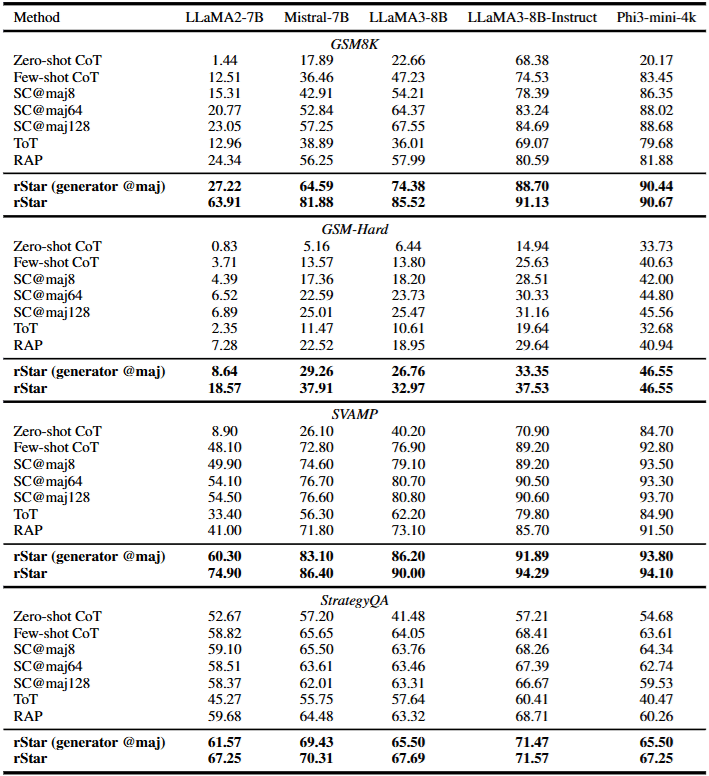
rStar (generator @maj) represents performing 32 Rollouts purely with the Generator and deciding the Final Answer via Majority Voting (without using the Discriminator at all).

From the table above, we can see that even without using the Discriminator for Mutual Reasoning, rStar still outperforms Baseline methods, indicating the Generator designed in rStar is effective. Adding the Discriminator for Mutual Reasoning significantly boosts performance further.

Reading the experimental data, I had a question:

Simple SC (Self-Consistency)@maj64 actually achieves decent performance. If rStar’s average LLM Calls per task are far higher than 64, and the performance gain isn’t much higher than SC@maj64, isn’t the method less cost-effective?

Actually, the paper honestly lists this data in Table 7 of Appendix A.2.

• Specific LLM Call counts, based on paper data (taking GSM8K as example):
  • LLaMA2-7B: Average 166.81 calls.
  • Mistral-7B: Average 148.90 calls.

Where do these ~150-160 LLM Calls come from?

1. Generator (MCTS): To generate 32 full Trajectories, although MCTS only does 32 Rollouts, due to Expansion (generating Actions) and Simulation (completing paths), plus the branching structure, it consumes about 120-130 calls on average.
2. Discriminator: Verifying the 32 generated paths requires a fixed 32 calls.
3. Total: $120 + 32 \approx 150+$ calls.

rStar’s cost is about 2.3 ~ 2.6 times that of SC@64 (close to SC@128 or SC@192 levels).

Besides LLM Call counts, the paper mentions an even more startling number: Generated Tokens.

• rStar generates an average of 360k (367.1k) Tokens per problem.
• This is because MCTS paths are often long (multi-step reasoning, sub-problems), plus the Discriminator reads long Contexts.

In comparison, if SC@64 has 200 tokens per path, the total is only 12.8k tokens. rStar’s Token cost is about 20~30 times that of SC@64.

However, we must look at “Return on Investment (ROI),” i.e., how much accuracy gain these added costs buy. This depends on the model’s base capability.

• Scenario A: Weak SLMs —— rStar wins hands down (Take LLaMA2-7B as example (Table 2)):
  • SC@64: Accuracy 20.77%
  • SC@128: Accuracy 23.05% (Even doubling to 128 calls, improvement is minimal)
  • rStar (~160 calls): Accuracy 63.91%

Conclusion: In this case, rStar’s benefit is huge. Why? Because weak models have serious “systematic errors.” SC@64 just repeats wrong logic 64 times (Garbage In, Garbage Out). rStar, through MCTS Action guidance, pushes the model’s capability boundary, solving problems SC cannot solve by stacking numbers. The cost increase here is very worthwhile.

• Scenario B: Stronger SLMs —— Gap narrows (Take LLaMA3-8B-Instruct as example)
  • SC@64: Accuracy 83.24%
  • rStar: Accuracy 91.13%

Conclusion: Improvement of about 8%. This depends on the application scenario. If you pursue extreme accuracy (improving from 83 to 91), 2.5x cost is acceptable. But if resources are limited, SC@64 is good enough.

Summary of choice between rStar and Self-Consistency:

1. Solving “Unsolvable” Problems: rStar’s real value is “help in a crisis.” When the model lacks capability (like LLaMA2-7B on math), sampling more with SC is useless. rStar makes the model “smarter,” which SC cannot do.
2. Solving “Careless” Problems: When the model is already strong (like GPT-4 or LLaMA3) and just occasionally careless, SC typically has better ROI.
3. Verdict: rStar’s benefit lies in mining the SLM’s potential upper limit, not just saving money. If your task is hard for the SLM (<50% accuracy), rStar is powerful; if it’s easy, SC suffices.

This is a hot topic in AI: Weak-to-Strong Generalization. We discussed the Discriminator’s role. Intuitively, we might think: “To check LLaMA3-8B’s answers, shouldn’t the discriminator be at least the same level?”

But in the table above, the authors conducted an interesting experiment:

• Generator: LLaMA3-8B-Instruct
• Discriminator: Switched between different models.

The result is surprising:

• Using Phi-3-Mini (3.8B) as discriminator: Accuracy 91.13%
• Using GPT-4 (Super Strong) as discriminator: Accuracy 92.57%

Interpretation: This shows rStar’s Mutual Consistency mechanism is robust. Even a discriminator much weaker than the Generator (3.8B vs 8B), as long as it can perform basic logical completion, can effectively filter correct answers. This is great news for lowering deployment costs (you can use a tiny model to monitor a larger one).

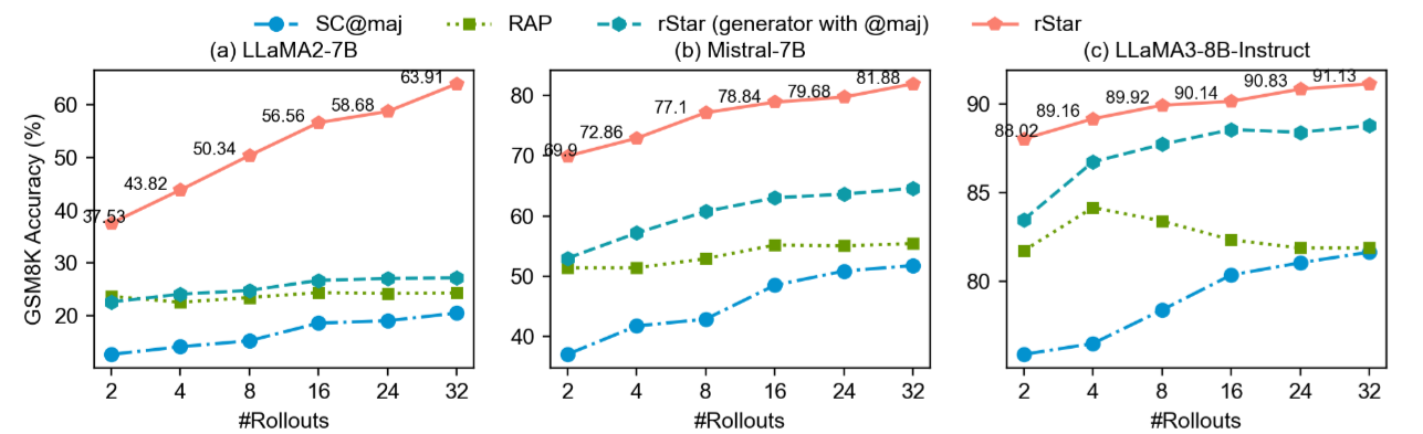
We just discussed rStar’s high cost (32 rollouts). But looking at the table above reveals a great trend.

Phenomenon:

• When Rollout count is only 2 (2 Rollouts), rStar significantly outperforms other Baselines (like RAP and SC).
• The curve saturates around 8~16 Rollouts; further improvement slows down.

This addresses our cost concern. Although the paper sets it to 32, in practice, we could cut Rollouts to 4 or 8. This would drastically reduce LLM Calls (maybe just slightly more than SC) while still enjoying MCTS’s structured reasoning advantages. This proves high-quality trajectories generated by rStar can be found very early.

We spent a lot of time discussing those 5 Actions ($A_1 \sim A_5$). You might ask: “Do we really need such complexity? Can’t we just use one move?”

The table above gives the answer (using LLaMA3-8B):

• Only $A_3$ (like RAP): 70.5%
• Only $A_3 + A_5$: 72.5%
• All ($A_1 \sim A_5$): 75.0%

This proves the value of a “Rich set of human-like reasoning actions.” A single decomposition strategy (like RAP) is useful but lacks flexibility for diverse problems. Adding “Rephrase ($A_5$)” and “One-step/Multi-step toggle ($A_1/A_2$)” indeed covers more reasoning blind spots. This also reminds us that future research could focus on designing even more diverse reasoning actions.

5 Conclusion

Finally, summarizing the three most important core concepts of this paper:

1. Inference Scaling Laws: This paper proves that besides stacking compute at the training end (Pre-training/Fine-tuning), we can also stack compute at the inference end (via Search and Verification) to massively boost model capabilities. This is a path to strength without retraining.
2. Mutual Reasoning: “Self-verification” is hard, but “Mutual verification” (fill-in-the-blank test) is effective. This method via Consistency rather than direct Scoring is a clever solution to the difficulty of training Reward Models.
3. MCTS as a Prompting Driver: Traditional MCTS is for games; rStar turns it into a Prompt scheduler. This demonstrates the powerful potential of combining Classic Algorithms with LLMs.