Is RLHF Killing Creativity? How Verbalized Sampling Mitigates Mode Collapse and Unlocks LLM Diversity

1 Introduction

In current AI research, we often observe a frustrating phenomenon: models that undergo fine-grained alignment (such as RLHF or DPO), while becoming safer and more obedient, also become “more boring.” Their creativity seems to be stifled, and their outputs are often monotonous. The paper Verbalized Sampling: How to Mitigate Mode Collapse and Unlock LLM Diversity offers a brand-new perspective on this issue.

Unlike past approaches that blamed algorithmic defects, this paper points out that the root of the problem lies in the data—specifically, the Typicality Bias in human preference data. To overcome this, the authors propose a training-free inference strategy: Verbalized Sampling (VS).

In this article, we will step through the paper’s derivation to understand why models “collapse” and how to “awaken” the suppressed diversity of models through simple prompting techniques.

2 Problem Definition: Why Does Model Diversity Decline?

2.1 Core Phenomenon: Mode Collapse

First, we need to define Mode Collapse. After post-training, the probability distribution of a model’s output becomes extremely sharpened. This causes the model to tend towards repeatedly outputting a very small number of “safe bets” or “standard answers,” which correspond to the Mode of the distribution.

2.2 Theoretical Attribution: Typicality Bias

The paper proposes a bold hypothesis: Humans have an innate cognitive bias, tending to give higher scores to text that “looks familiar” and “matches intuition.”

This innate human bias is reflected in the Preference Dataset we construct. Consequently, the Reward Model trained on this dataset acquires this bias, and the language model post-trained based on this Reward Model learns it as well.

To quantify this, the authors established a mathematical model for the Reward Model:

• $r(x, y)$: The total reward given by humans.
• $r_{\text{true}}(x, y)$: The objective score of the real task (e.g., correctness, instruction compliance).
• $\log \pi_{\text{ref}}(y \mid x)$: The Log-Likelihood of the pre-trained model (Base Model).
• $\alpha$: The Typicality Bias Coefficient.

Why do the authors use the Base Model ($\pi_{\text{ref}}$) to represent typicality?

This is based on a key assumption by the authors: The pre-trained model (Base Model) is trained on massive amounts of human text, so it captures the statistical laws and distributions of human language. In other words, if a sentence has a high probability (High Log-likelihood) in the Base Model, it implies that the sentence fits human daily usage habits very well and is very “typical.” Therefore, the authors use the Base Model’s Log-likelihood as the best mathematical proxy for the “sense of familiarity” and “typicality” in the human mind.

2.2.1 Verifying $\alpha > 0$: Controlled Variable Experiment

To prove that $\alpha$ actually exists, the authors used the HelpSteer dataset for experiments. The experimental design is very ingenious:

1. Select Response Pairs with identical Correctness. This means the influence of $r_{\text{true}}$ is eliminated.
2. Observe which of the two humans tend to consider more Helpful.
3. Use the Bradley-Terry Model for regression analysis to estimate $\alpha$.

The experimental results show that $\alpha \approx 0.6$, confirming that the Preference Dataset labeled by humans indeed significantly favors typical content, and our current Reward Models also learn this bias.

2.3 Mathematical Proof: How Bias Leads to Collapse

Knowing that $\alpha > 0$, how does this lead to Mode Collapse? Let’s derive it step by step.

2.3.1 RLHF Optimization Objective

The goal of RLHF is to maximize Reward while limiting the KL divergence from the Base Model to prevent model degradation:

Where $\beta$ is the KL penalty coefficient.

2.3.2 Closed-Form Solution

According to reinforcement learning theory, the optimal solution $\pi^*$ for the above objective function has the following Closed-Form Solution:

2.3.3 Substituting the Biased Reward Function

Now, we substitute the biased Reward function $r(x, y) = r_{\text{true}} + \alpha \log \pi_{\text{ref}}$ verified earlier into the equation above:

2.3.4 Merging using Logarithmic Rules

Using the mathematical property $e^{k \log x} = x^k$, we can transform the last term: $\exp\left( \frac{\alpha}{\beta} \log \pi_{\text{ref}} \right) = \pi_{\text{ref}}^{\frac{\alpha}{\beta}}$.

Then merge all $\pi_{\text{ref}}$ terms:

2.3.5 Defining $\gamma$ and Conclusion

We define the scaling coefficient $\gamma = 1 + \frac{\alpha}{\beta}$, finally obtaining:

2.3.6 Key Conclusion

Since $\alpha > 0$ (Typicality Bias exists) and $\beta > 0$, it follows that $\gamma > 1$. This means we are taking the probability distribution of the Base Model to a power greater than 1. Mathematically, this leads to the strong getting stronger, and the weak getting weaker (e.g., $0.9^2=0.81$, $0.1^2=0.01$, the gap widens).

This is the mathematical essence of Mode Collapse: The distribution is extremely “sharpened,” forcing the model to collapse onto the Mode with the highest probability.

3 Method: Verbalized Sampling (VS)

Since the problem is that the distribution after RLHF is too sharp, can we let the model “restore” this distribution itself? The authors propose Verbalized Sampling.

3.1 Core Insight: Different Prompts Collapse to Different Modes

The authors categorize Prompting into three levels:

1. Instance-level (Traditional phrasing): “Tell me a joke.” -> The model samples directly, constrained by $\gamma$, and will only output the most common joke.
2. List-level (List phrasing): “Tell me 5 jokes.” -> The model performs sequence generation. Since it is still greedily searching for high-score areas and implies a uniform distribution assumption, it often lists 5 very similar variants. This does not solve Mode Collapse.
3. Distribution-level (VS): “Generate 5 jokes and their probabilities.” -> This is the core of this paper.

3.2 Core Mechanism: Verbalize Probabilities

When we ask the model to “verbally state probabilities,” the model’s task changes from “Sampling” to “Describing.”

• The model is forced to call upon underlying knowledge to estimate the distribution, which effectively bypasses the sharpening effect of RLHF.
• Theoretical proof (see the paper’s Appendix) shows that the distribution reconstructed in this way can highly approximate the original distribution from the pre-training stage (Pre-training).

Here are the three main VS Prompt patterns:

3.2.1 VS-Standard

The most general, basic version, suitable for most tasks.

You are a helpful assistant.

Instruction:
Generate 5 responses to the input prompt: "{input_prompt}"

Format Requirements:
Return the responses in JSON format with the key: "responses" (a list of dictionaries). Each dictionary must include:
1. "text": the response string itself.
2. "probability": the estimated probability of this response (from 0.0 to 1.0) given the input prompt, relative to the full distribution of possible responses.

Input Prompt:
{input_prompt}

3.2.2 VS-CoT (Chain-of-Thought)

Combines Chain-of-Thought, letting the model think about diversity strategies first, then generate the distribution. Suitable for complex writing tasks.

Instruction:
Generate 5 responses to the input prompt using chain-of-thought reasoning.

Step 1:
Provide a "reasoning" field. Analyze the request and think about different angles, styles, or perspectives to ensure diversity in the responses.

Step 2:
Generate the responses in JSON format with the key "responses". Each item must include:
- "text": the response string.
- "probability": the estimated probability relative to the full distribution.

Input Prompt:
{input_prompt}

3.2.3 VS-Multi (Multi-turn Dialogue)

Excavates the long-tail distribution through multi-turn dialogue. After the first round of generation, the results are put into history, and the second round requests “different” content.

System:
(Keep previous context)

User:
Generate 5 MORE alternative responses to the original input prompt. These should be distinct from the previous ones.

Format Requirements:
Return the responses in JSON format with the key "responses", including "text" and "probability" (relative to the full distribution).

4 Experimental Results

We focus on four sets of key experimental data to verify the effectiveness of VS.

4.1 Diversity-Quality Trade-off

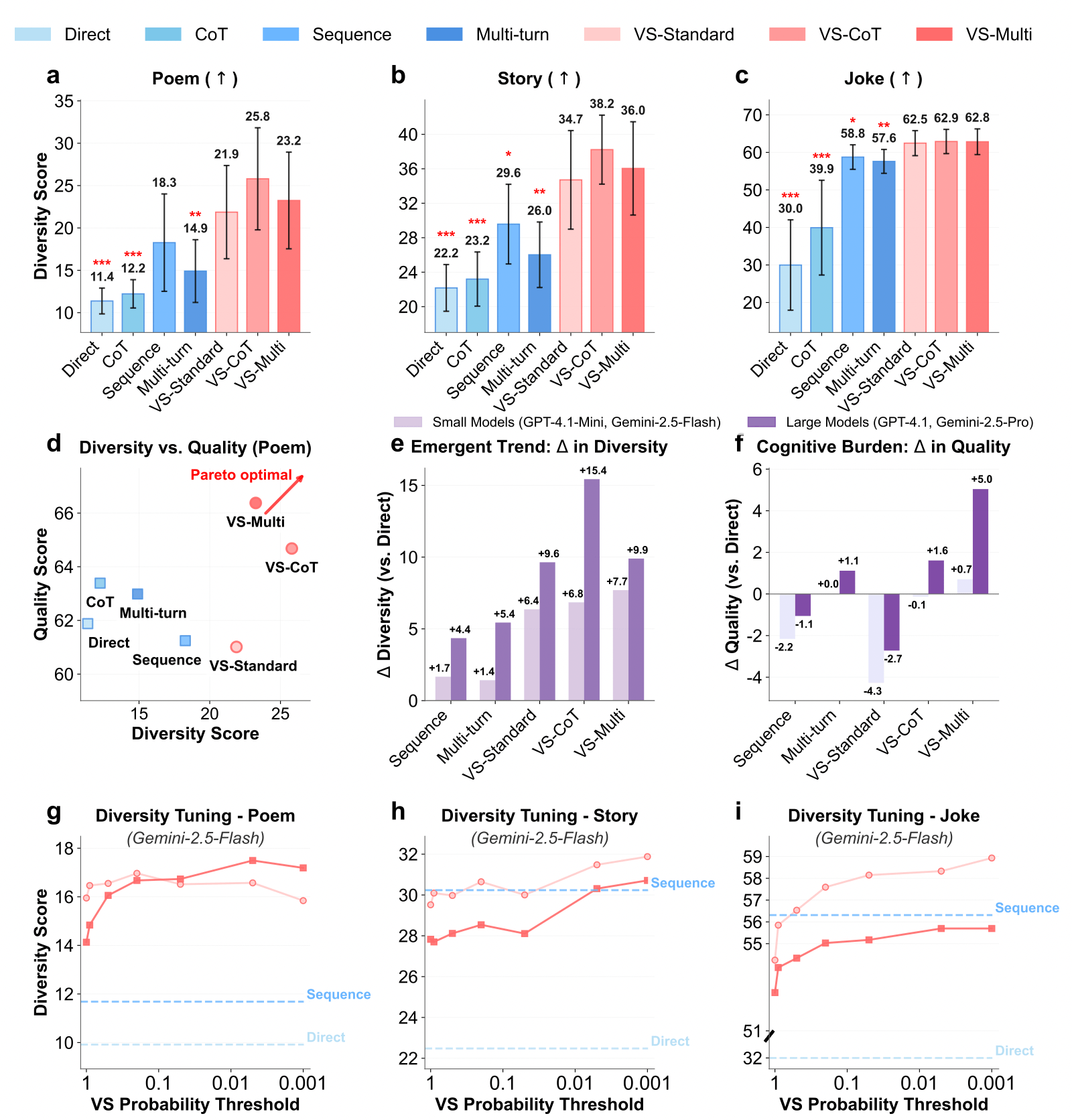
• Pareto Front: In Figure 4(d), VS-CoT (red line) pushes the entire curve to the upper right. This implies that VS provides higher diversity for the same level of quality.
• Human Evaluation: In the Joke task, the diversity score for VS (3.01) is significantly higher than direct questioning (1.83).
• Emergent Trend: As shown in Figure 4(e), stronger models (like GPT-4.1) gain far more diversity from VS compared to smaller models (like GPT-4.1-mini), proving that this method relies on the model’s instruction following and calibration capabilities.

4.2 Theoretical Verification: Restoring the Pre-training Distribution

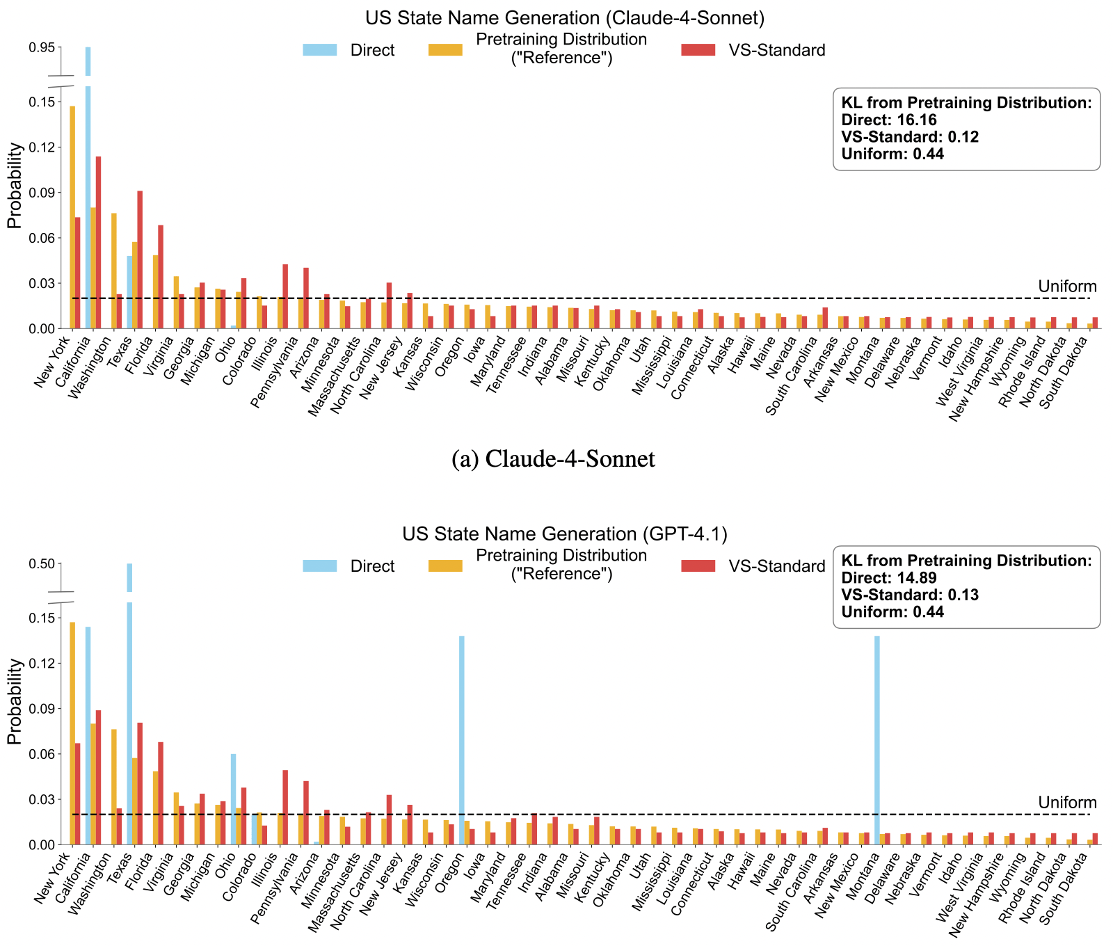
In the “Name a US State” experiment, the authors calculated the KL Divergence between the generated distribution and the true pre-training data distribution.

• Direct Prompting: KL $\approx 14.8$ (Severe collapse)
• VS-Standard: KL $\approx 0.13$ (Almost perfect restoration) This directly confirms that VS can successfully awaken the knowledge distribution suppressed within the model.

4.3 Downstream Application: Synthetic Data Generation

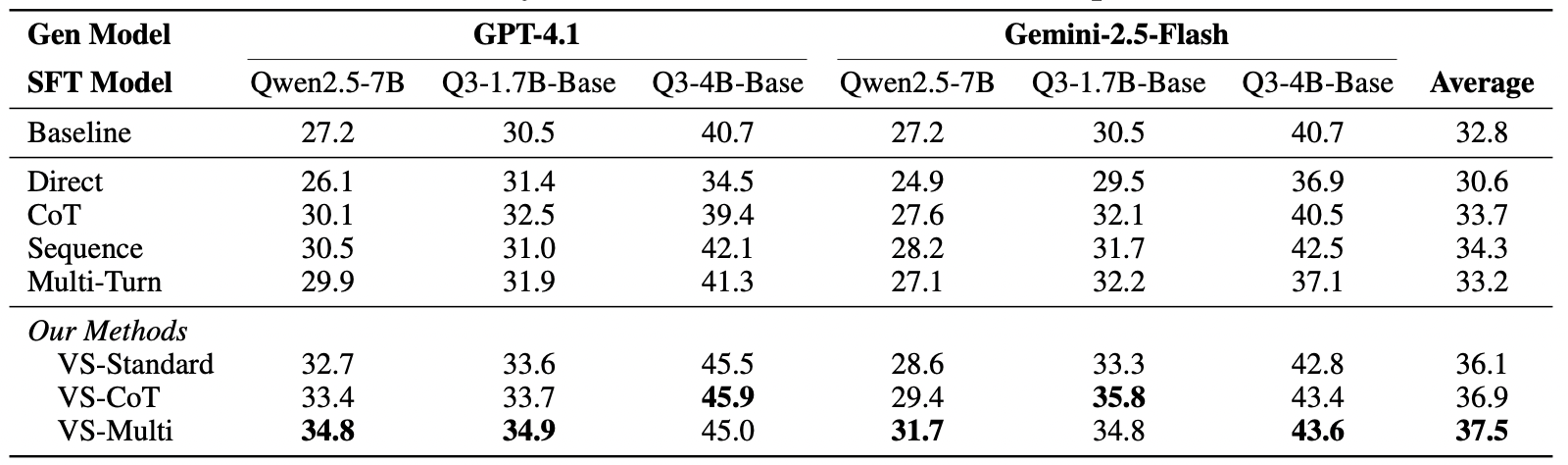
VS can not only write poems but also improve mathematical capabilities.

• Experimental Design: Use VS to generate math problems to fine-tune a small model.
• Results show that compared to the Baseline (30.6%), accuracy improved to 37.5% after fine-tuning with data generated by VS-Multi. This proves that data generated by VS possesses high quality and high coverage, making it extremely valuable for the field of Data Synthesis.

5 Conclusion

The most important insight this paper brings us is: A model’s “mediocrity” and “lack of creativity” are often not because it lacks the ability, but because it tries too hard to cater to human “Typicality Bias.”

Through Verbalized Sampling, we do not need expensive retraining. We only need to change the way we communicate with the model—shifting from simply “demanding answers” to “exploring possibilities”—to unlock the deep creative potential of LLMs. This offers a highly potential direction for future inference acceleration, data synthesis, and creative auxiliary tools.